Blog
RedisTimeSeries Version 1.2 Is Here!
When you think about it, “life is a time series.”
So maybe it shouldn’t be surprising that even though the RedisTimeSeries module—which simplifies the use of Redis for time-series use cases like IoT, application monitoring, and telemetry—has been generally available only since June of 2019, we are already seeing a large number of interesting use cases. For example, the New York Times is using RedisTimeSeries in its internal Photon project, as is Amazon Web Service’s IoT Greengrass project (see the GitHub repo here).
But we’re not here to rest on our laurels. Instead, we’re announcing general availability of a major new version of the module, RedisTimeSeries 1.2, which debuts with a long list of powerful new features. But given the widespread interest, our main goal for RedisTimeSeries 1.2 was to increase usability without degrading performance. Because Redis is an in-memory database, storing a large volume of time-series data in DRAM can become expensive. So in version 1.2 we added compression that reduces its memory requirements up to 90% in most scenarios—in theory, it could compress your time series data by up to 98%! We made our API more consistent and intuitive, and removed redundant response data to further improve performance. Together, the API changes and the compression improves read performance up to 70%. Put it all together and the new version of RedisTimeSeries could save users serious money on infrastructure costs without affecting performance.
(Check out our companion blog post on RedisTimeSeries 1.2 Benchmarks for more info on how ingestion throughput is independent of the number of time series in the dataset, of the compression, and of the number of samples in a time series.)
But let’s start with how the compression works, because it’s kind of cool.
Gorilla compression
A time series in RedisTimeSeries consists of a linked list of chunks that each contain a fixed number of samples. A sample is a tupleof a timestamp and a value representing a measurement at a specific time. Time is represented as a timestamp and the value as a float (double-precision floating point format). The chunks themselves are indexed in a Radix tree. You can read more about the internals here.
Uncompressed, the timestamp and the value each consume 8 bytes (or 16 bytes/128 bits in total) for each sample. For the timestamps we use double-delta compression and for the values we use XOR (“Exclusive or”) compression. Both techniques are based upon the Facebook Gorilla paper and are documented in our source code, but we’ll explain how it works below.
Double-delta encoding of the timestamp
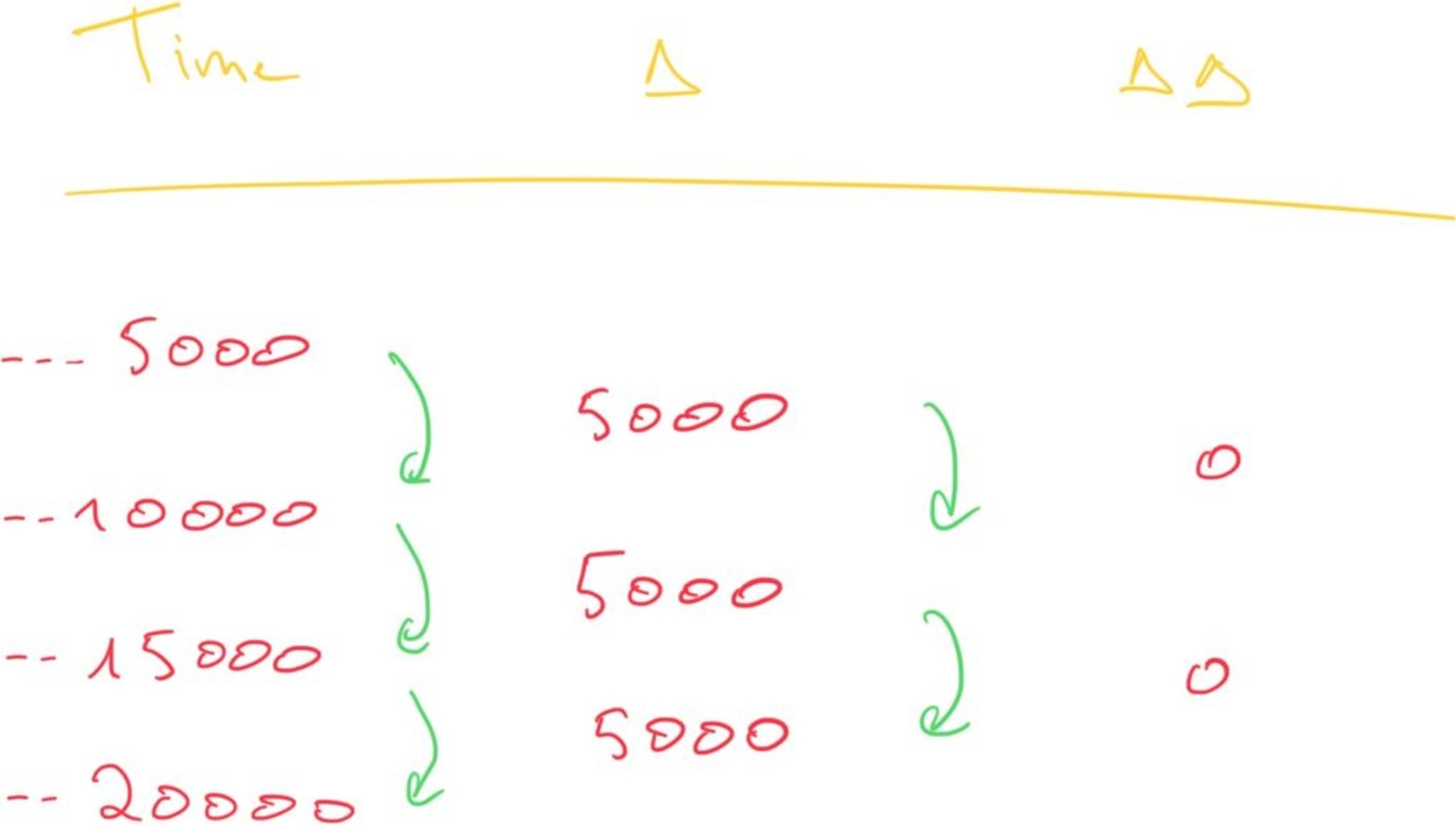
In many time-series use cases, samples are collected at fixed intervals. Imagine we are collecting measurements from a temperature sensor every 5 seconds. In milliseconds, the delta between two consecutive samples would be 5,000. Because the intervals remain constant, however, the delta between two deltas—the double-delta—would be 0.

Occasionally data will arrive at second 6 or second 4, but usually this is the exception. Rather than storing this ΔΔ (double-delta) in its entirety in 64 bits, variable-length encoding is used according to the following pseudo code:
If ΔΔ is zero, then store a single ‘0’ bit
Else If ΔΔ is between [-63, 64], store ‘10’ followed by the value (7 bits)
Else If ΔΔ is between [-512,511], store ‘110’ followed by the value (10 bits)
Else if ΔΔ is between [-4096,4095], store ‘1110’ followed by the value (13 bits)
Else if ΔΔ is between [-32768,32767], store ‘11110’ followed by the value (16 bits)
Else store ‘11111’ followed by D using 64 bits
XOR compression of the value
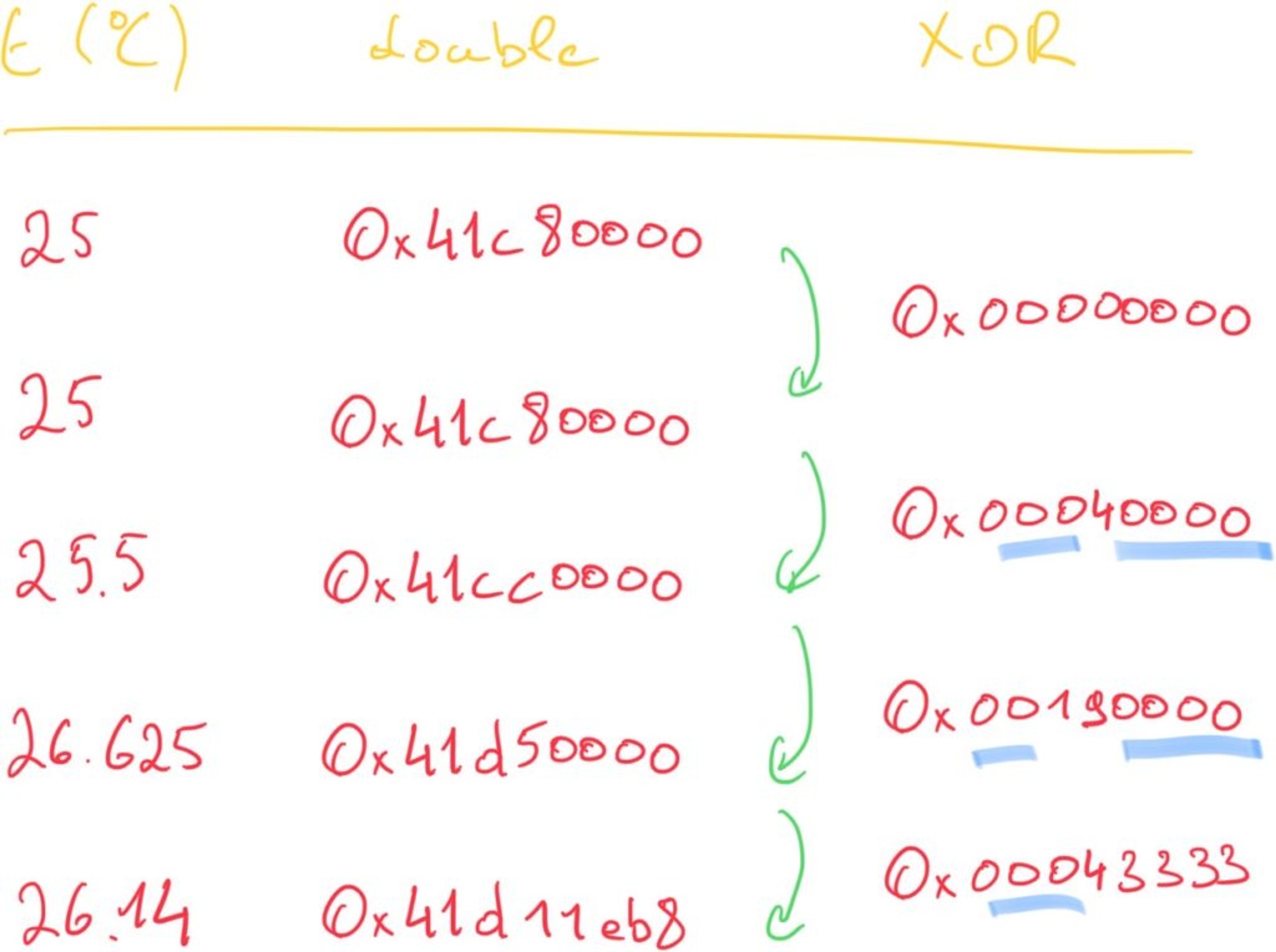
The basis of the value compression is the assumption that the difference between consecutive values is typically small and happens gradually instead of abruptly. In addition, floats are inherently wasteful and contain many repeating zeros that can be eliminated. So, when two consecutive values are XORed, only a few meaningful bits will be present in the result. For simplicity, the example below uses a single-precision double—RedisTimeSeries uses double-precision doubles:

You can see that the XOR operation between the first two equal numbers is, obviously, 0. But also there are often a number of leading and trailing 0s around the meaningful XOR value. The variable-length encoding of the XOR differences of the values removes leading and trailing zeros.
There is also a control bit that can further reduce the number of bits consumed by a sample. If the block of meaningful bits falls within the block of the previous value’s meaningful bits, i.e., there are at least as many leading zeros and as many trailing zeros as in the previous value, then the number of leading and trailing zeros of the previous sample can be used:
If XOR is zero (same value)
store single ‘0’ bit
Else
calculate the number of leading and trailing zeros in the XOR,
store bit ‘1’ followed by
If the block of meaningful bits falls within the block of previous meaningful bits,
store control bit `0`
Else store control bit `1`,
store the length of the number of leading zeros in the next 5 bits,
store the length of the meaningful XOR value in the next 6 bits.
Finally store the meaningful bits of the XOR value.
Resulting memory consumption
So how much memory reduction can this technique give you? Not surprisingly, the actual reduction depends on your use case, but we noticed a 94% reduction in our benchmark datasets. According to page six of Facebook’s Gorilla paper, each sample consumes an average of 1.37 bytes, compared to 16 bytes. This results in a 90% memory reduction for the most common use cases.
The theoretical limit is reached when the double-delta is 0 and the XOR is also 0. In that case, each sample uses 2 bits instead of 128, resulting in a memory reduction of 98.4%! In the worst case scenario, a sample consumes 145 bits: 69 bits for the timestamp and 76 bits for the value. (For this extreme case to happen, the double-delta would have to be over MAX_32 and float values would be extremely complex and different. Because we don’t want to exclude even extreme use cases, you can still use the `UNCOMPRESSED` option when you create a time series.)
API enhancements
Time-series use cases are mainly append-only, which allows for optimizations such as the compression described above. But with this compression approach, inserting a sample with a timestamp earlier than the last sample will not only introduce more complex logic and consume more CPU cycles but also require more complex memory management.
That’s why with RedisTimeSeries 1.2, we made the API more strict and no longer allow clients to rewrite the last sample of the time series. That might sound limiting, but most of the changes are intuitive and actually enhance the developer experience.
As a consequence, the automatic calculation of the aggregated sample for a downsampled time series now happens at the source time series. Only when the aggregation time window has passed, will the sample representing the aggregation be written to the downsampled time series. This means that writes happen less often to the downsampled time series, further enhancing ingestion performance.
With downsampling, you can reduce your memory consumption by aggregating samples that lay further in the past. But you can also model counters for time windows of fixed sizes, for example the number of website pageviews per hour. You can construct these counters easily with RedisTimeSeries. In the source time series you use TS.ADD to add a sample with the value you would like the counter to be incremented and a downsampling rule with a sum aggregation over the fixed window size:
redis:6379> TS.CREATE ts RETENTION 20000
OK
redis:6379> TS.CREATE counter
OK
redis:6379> TS.CREATERULE ts counter AGGREGATION sum 5000
OK
redis:6379> TS.ADD ts * 5
(integer) 1580394077750
redis:6379> TS.ADD ts * 2
(integer) 1580394079257
redis:6379> TS.ADD ts * 3
(integer) 1580394085716
redis:6379> TS.RANGE counter - +
1) 1) (integer) 1580394075000
2) "7"
redis:6379> TS.ADD ts * 1
(integer) 1580394095233
redis:6379> TS.RANGE counter - +
1) 1) (integer) 1580394075000
2) "7"
2) 1) (integer) 1580394085000
2) "3"
redis:6379> TS.RANGE ts - +
1) 1) (integer) 1580394077750
2) "5"
2) 1) (integer) 1580394079257
2) "2"
3) 1) (integer) 1580394085716
2) "3"
4) 1) (integer) 1580394095233
2) "1"
redis:6379>
In both cases the downsampled series will have the exact counter you’re looking for.
What’s next for RedisTimeSeries?
The addition of Gorilla compression and API enhancements have dramatically reduced memory consumption. (For more information on how this works, see the companion blog post on RedisTimeSeries 1.2 Benchmarks.)
But we’re not done yet. Looking forward, we plan to replace the RedisTimeSeries proprietary secondary indexing using sorted sets with the new low-level API used in RediSearch. This will let users do full-text search queries on the labels linked the time series using a rich and proven query language. We are also working to complete our API to be in line with other Redis data structures by introducing the TS.REVRANGE and TS.MREVRANGE commands.
Most Redis modules focus on solving one particular problem extremely well and extremely quickly—combining them enables a large set of interesting new use cases. We are currently exploring combining RedisTimeSeries and RedisAI to do real-time anomaly detection and unsupervised learning. Lastly, we are working to expose a low-level API for RedisGears that will allow you to do cross-time series aggregation in the most performant way.
Get started with Redis today
Speak to a Redis expert and learn more about enterprise-grade Redis today.
