Blog
Unlocking Time-Series Data with Redis
(Note: This blog post was adapted from a webinar I presented in June. To go even deeper into RedisTimeSeries, register and watch the webinar now!)
Most developers know that Redis real-time response capabilities makes it well suited for working with time-series data. But what exactly is time-series data? Plenty of definitions stretch into page after page of explanation, but I think it can be dramatically simplified:
Basically, time-series data is data that encodes time as an index, and where each recorded time has a numeric value. If you visualize it in two columns, one column would have some sort of time index, usually timestamps in the Unix epoch form. And the other column would have some sort of numeric value.
Very simple.
Critically, you can analyze time-series data using time bounds, for example, to see happened between January 1st and January 3rd. You can also get granular, into seconds, sometimes even milliseconds. You can also separate your data into time units, to see what happened on an hourly basis. Then, if you don’t want to look at every single event in your time-series data, you can put an aggregation on top of that, to get averages per hour, for example.
Many people picture stock charts when they think of time-series data. It’s a good way to look at how a stock performed during a given time period. One time-series data use case that I look at a lot is the CPU load on a server during any specified interval. Time-series data is also a good way to look at sensor data and other Internet of Things (IoT) information. Any time you’re looking at trends over time, that’s usually sourced in some sort of time-series database or time-series structure.
The history of Redis and time-series data
Now let’s focus on Redis and time series. It all started with Sorted Sets, one of the built-in data structures in Redis. People started using Sorted Sets for time-series data early on, looking something like this:
> ZADD mySortedSet 1559938522 1000
This example includes the ZADD command, mySortedSets as the key, and a timestamp, which as the score. And finally the member, which was the value.
That was great, but you could get only ranges, you couldn’t do averages or downsampling.
Sets cannot have repeats. Here, if you have two different timestamps with the same value, the set is based on the member (in this case what we’re defining as the value.) So in the example below, the second one would actually be an upsert—it would overwrite the first one. That doesn’t work for time-series data and people had some rude awakenings when they used it that way:
> ZADD mySortedSet 1559938522 1000
> ZADD mySortedSet 1559938534 1000
Developers came up with a number of workarounds that were computationally complex and really hard to implement. There had to be an easier way.
Enter Redis Streams
Then, about two years ago, Redis 4.0 debuted with Redis Streams, which was designed to solve problems in building applications with the unified log architecture and for interprocess messaging.
Redis Streams offered important advantages over Sorted Sets for time-series use cases. It allowed for auto-generated IDs, no duplicates, and per-sample field/value pairs.
> XADD myStream * myValue 1000
> XADD myStream * myValue 1000 anotherField hello
As you can see in the first command, we set the field myField to 1000. In the second command a new entry was created with myValue set to 1000 as well as anotherField set to hello. Each of these are entries in the stream located at the key myStream.
But this still lacked important features and wasn’t really designed for time-series data. You can easily get time ranges, but not a whole lot else.
Now let’s rewind a bit to talk about the Redis modules API, which came out a little bit before Streams and allowed Redis to have additional communities and data types. Redis users could build modules that would act as first-class citizens inside Redis. Existing modules include everything from RediSearch to RedisGraph to RedisJSON. And now there’s RedisTimeSeries, which basically creates an entire time-series database inside Redis.
How the RedisTimeSeries module works
Before we get to how to use the RedisTimeSeries module, it’s important to understand what’s going on under the hood.
The first thing you need to learn about is ‘the chunk.’ You actually never manipulate a chunk directly, but RedisTimeSeries stores all the data in these chunks. Each chunk consists of two correlated arrays (one for timestamps and one for sample values) in a doubly linked list.
For example, let’s say I want to put a timestamp into my time-series database. It goes on the first row in the two arrays. If you have additional samples, they would just go into the array.

Chunks are a fixed size. When chunk is full, additional data automatically goes to the next chunk. Adding to the beginning or end of a linked list is computationally trivial, so when new chunks are added it is very lightweight.
But unlike most Redis data types, it’s best practice to first create your time-series key. In this case, my command is TS.CREATE. And then I have myTS, which is the key that I’m using here.
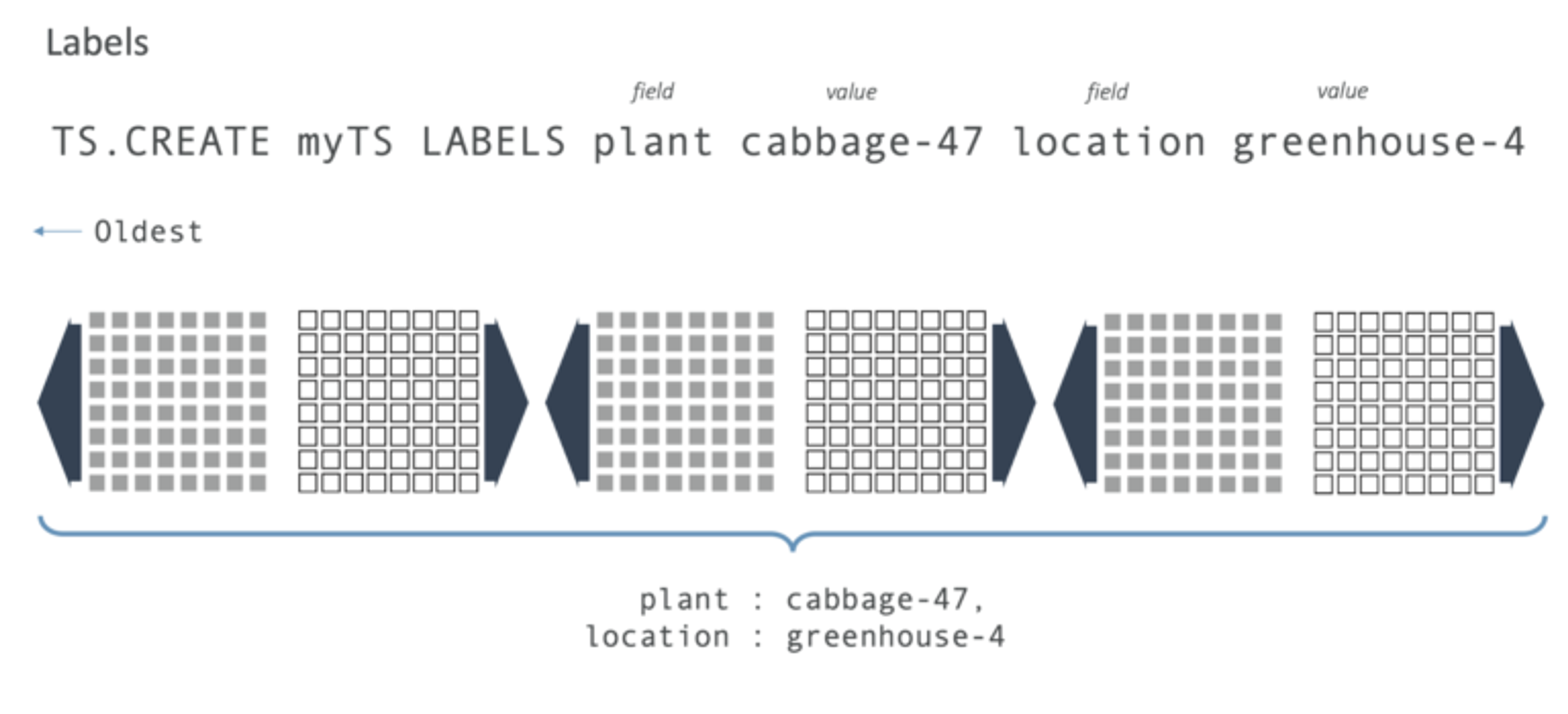
So let’s say that we want to add in some metadata to this key. Imagine we’re running a vegetable nursery and we want to track cabbage number 47 in greenhouse number 4; we would call this metadata labels. This would apply to every single sample across the entire time series:

Another important part of working with time-series data is retention. Let’s say that we don’t care about anything older than 60 seconds. RedisTimeSeries can trim off things that are outside the retention time periods you specify.
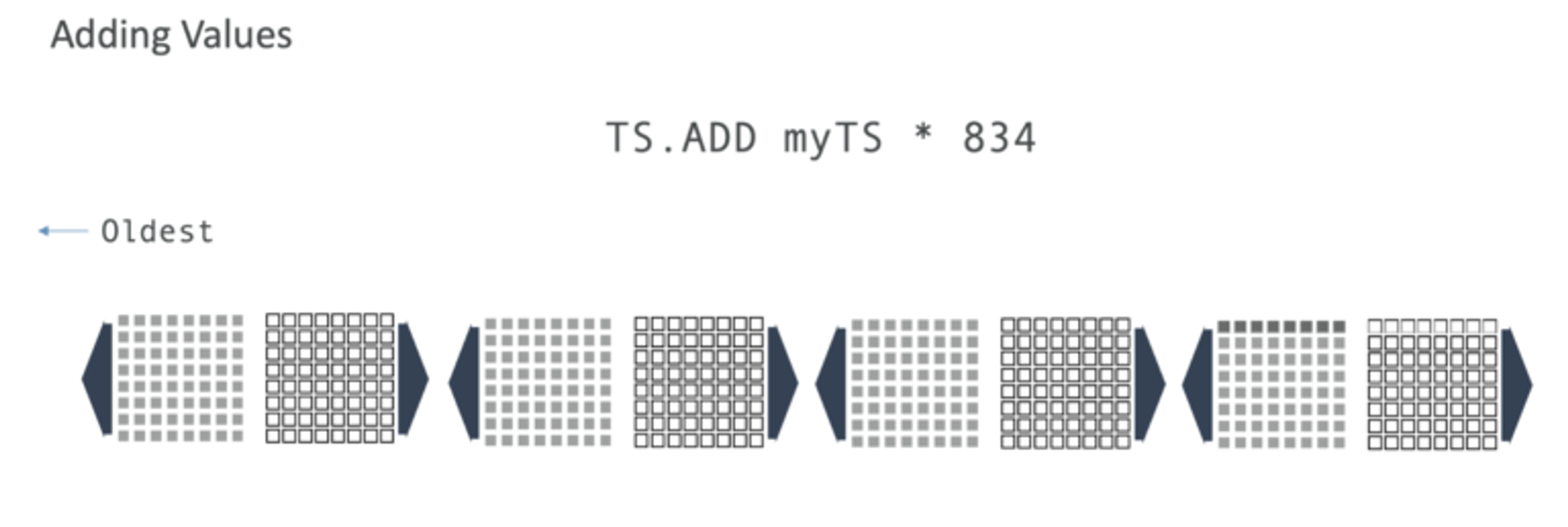
We can add values using an operation called TS.ADD. The first argument is the key myTS and the asterisk is syntax borrowed from Redis Streams indicating that Redis will auto generate the timestamp. In this case, the value is 834.

Lets let’s add another sample, and specify a timestamp. Note that timestamps are effectively append-only, so you can’t go in and add something past the most recently used timestamp. The subsequent TS.ADD would have to be a timestamp greater than that value.
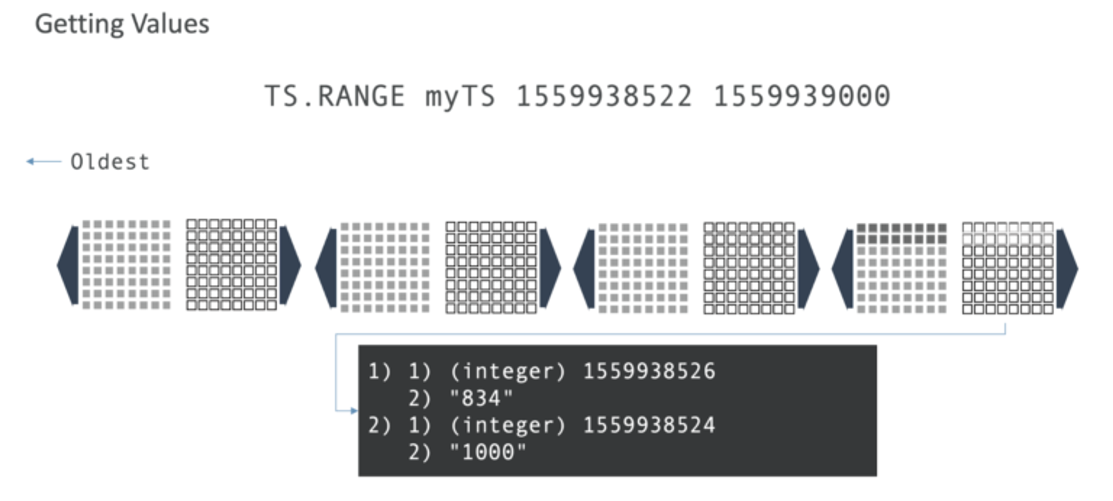
Next, to get bounded results, you would ask for all the samples between the two timestamps. Using our example, you can see the first timestamp has a value of 834 and the second one has 1000.
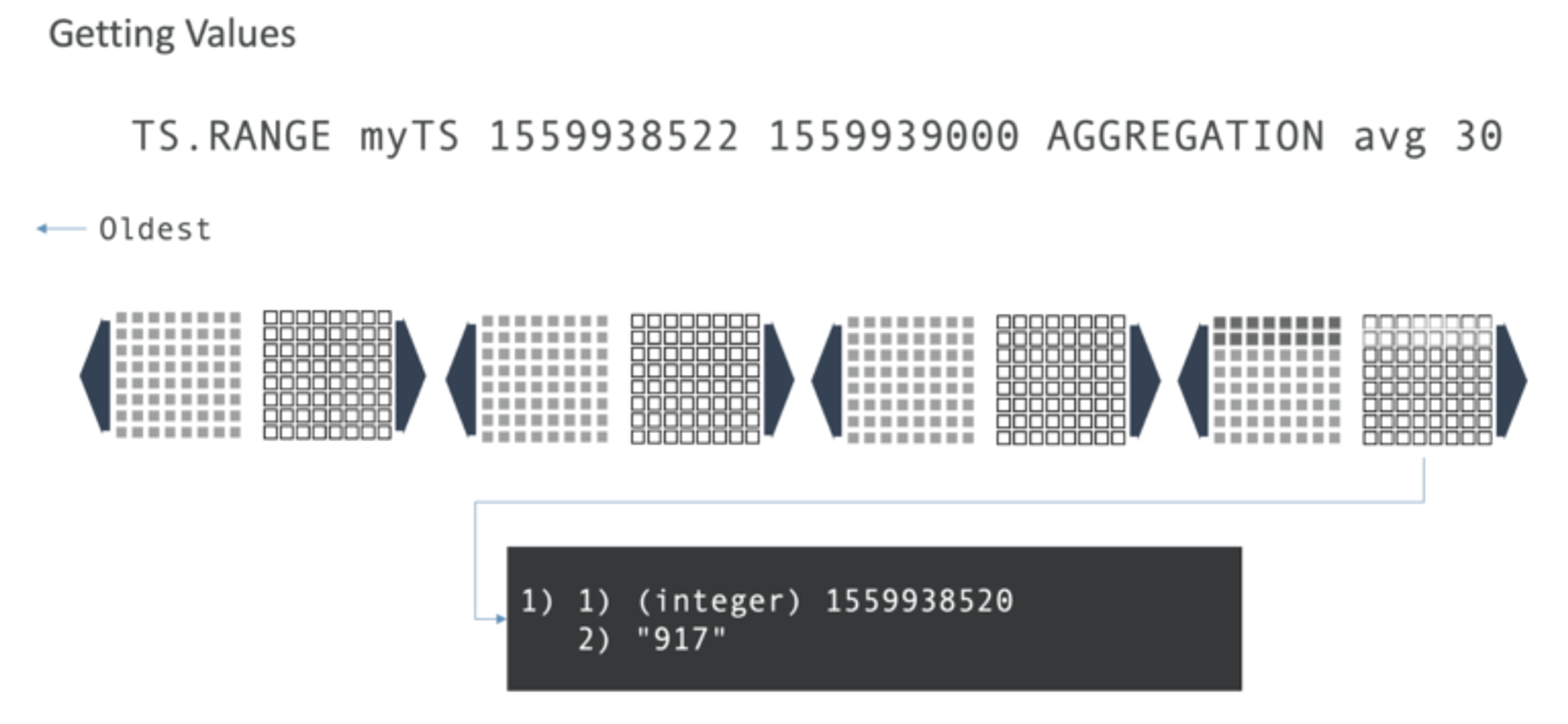
That’s useful, but maybe you want the average for every 30-second time period. Here, avg is is our keyword and the 917, of course, is the average of 834 and 1,000.

But what happens when you have a lot more data? You might not want to run that TS.RANGE command all the time and just want to granularly extract that data.
Well, we have the ability to create rules! myTS is my key: That’s the source. The destination is myTS2 and that’s the second key. All the chunks here represent 30 seconds of time and RedisTimeSeries will automatically put that into the secondary key of destination Key. So as every 30 seconds passes, you’ll get one more sample added to myTS2.
But wait, there’s more! It’s not just limited to averages. You can sum, you can get the minimum, you can get the maximum, you can get a range. You can get the count—how many— and the first or the last. And all those different aggregation functions also apply for TS RANGE.
More commands for RedisTimeSeries
Let’s take a look at what else RedisTimeSeries can do. The commands TS.INCRBY and TS.DECRBY are for counting over time. TS.INCRBY increments the previous entry by some value. Let’s say you know that in 10 seconds you have collected 10 widgets. you would run TS.INCRBY on a key. In this way you don’t have to know the previous value and you can keep a running tally. The same applies for TS.DECRBY, only in reverse.
TS.GET, meanwhile, grabs the last value. And TS.ALTER lets you change the metadata for keys you have created, including fields, values retention, and more.
TS.MRANGE and TS.MGET are interesting but a bit complicated to explain. RedisTimeSeries tracks all the different time-series keys in the database. TS.MRANGE lets you specify a key/value pair of labels. So in our greenhouse example, you could get the temperature readings for Greenhouse 4 and then use TS.MRANGE to look at different keys across the entire keyspace. Similarly, TS.MGET lets you get the single most recent values by labels. You can connect RedisTimeSeries with different parts of your infrastructure, such as Prometheus and Grafana, which is a great way to power monitoring dashboards.
Caching RedisTimeSeries
Even as we find our customers using time-series data for more and more use cases, many companies are still storing their time-series type in relational databases. That’s simply not a great fit from a technology perspective when it comes to scaling things. It might work fine when just two or three people are looking at a dashboard, but when you want thousands of people throughout the organization to all look at the same analytical dashboard dashboards, ad hoc queries of a relational database often can’t keep up.
That’s why we see RedisTimeSeries being used to cache time-series data that would otherwise be used in a slower database, and also to get other Redis benefits, including the choice whether to persist your data or keep it ephemeral..
Want to learn more?
- Register and watch the Unlocking TimeSeries Data with Redis webinar now, including informative answers to real-world questions.
- Go to RedisTimeSeries.io and explore how to launch RedisTimeseries from Docker, check out all the available commands, or build it yourself.
- Visit Github.org (a single repo wasn’t enough, it also contains the module source code as well as connectors and examples!)
Get started with Redis today
Speak to a Redis expert and learn more about enterprise-grade Redis today.
