Blog
Count-Min Sketch: The Art and Science of Estimating Stuff
This post is about what are, in my opinion, two of the most exciting things in the world: probabilistic data structures and Redis modules. If you’ve heard about one or the other then you can surely relate to my enthusiasm, but in case you want to catch up on the coolest stuff on earth just continue reading.
I’ll start with this statement: large-scale low-latency data processing is challenging. The volumes and velocities of data involved can make real-time analysis extremely demanding. Due to its high performance and versatility, Redis is commonly used to solve such challenges. Its ability to store, manipulate and serve multiple forms of data in sub-millisecond latency makes it the ideal data container in many cases where online computation is needed.
But everything is relative, and there are scales so extreme that they make accurate real-time analysis a practical impossibility. Complex problems only become more difficult as they get bigger, but we tend to forget that simple problems follow the same rule. Even something as basic as summing numbers can become a monumental task once data is too big, too fast or when we don’t have enough resources to process it. And while resources are always finite and expensive, data is constantly growing like nobody’s business.
What is Count-min Sketch?
Count-min sketch (also called CM sketch) is a probabilistic data structure that’s extremely useful once you grasp how it works and, more importantly, how to use it.
Fortunately, CM sketch’s simple characteristics make it relatively easy for novices to understand (turns out many of my friends were unable to follow along with this Top-K blog).

CM sketch has been a Redis module for several years and was recently rewritten as part of the RedisBloom module v2.0. But before we dive into CM sketch, it is important to understand why you’d use any probabilistic data structure. In the triangle of speed, space, and accuracy, probabilistic data structures sacrifice some accuracy to gain space—potentially a lot of space! The effect on speed varies based on algorithms and set sizes.
- Accuracy: By definition, keeping only part of your data and allowing collisions in storage reduces accuracy. Yet you can set the maximum error rate based on your use case.
- Memory space: In a world of big data where billions of events are recorded, storing only partial data can tremendously reduce storage space requirements and costs.
- Speed: Certain traditional data structures operate relatively inefficiently, slowing response time. (For example, a Sorted Set maintains the order of all elements in it, but you might be interested in just the top elements. Because probabilistic algorithms maintain only a partial list, they are more efficient and can often answer queries much faster.
The right probabilistic data structure allows you to keep only part of the information in your dataset in exchange for reduced accuracy. Of course, in many cases (bank accounts, for example), reduced accuracy is unacceptable. But for recommending a movie or showing ads to website users, the cost of a relatively rare mistake is low and the space savings could be substantial.
Basically, CM sketch works by aggregating the count of all items in your dataset into several counter arrays. Upon a query, it returns the item’s minimum count of all arrays, which promises to minimize the count inflation caused by collisions. Items with a low appearance rate or score (“mouse flows”) have a count below the error rate, so you lose any data about their real count and they are treated as noise. For items with a high appearance rate or score (“elephant flows”), simply use the count received. Considering CM sketch’s size is constant and it can be used for an infinite number of items, you can see the potential for huge savings in storage space.
For background, sketches are a class of data structures and their accompanying algorithms. They capture the nature of your data in order to answer questions about it while using constant or sublinear space. CM sketch was described by Graham Cormode and S. Muthu Muthukrishnan in a 2005 paper called “An Improved Data Stream Summary: The Count-Min Sketch and its Applications.”
Count-min Sketch: What and how
CM sketch uses several arrays of counters to support its primary use cases. Let’s call the number of arrays “depth” and the number of counters in each array “width.”
Whenever we receive an item, we use a hash function (which turns an element—a word, sentence, number, or binary—into a number that can be used as a location in the set/array or as a fingerprint) to calculate the location of the item and increase that counter for each array. Each of the associated counters has a value equal to or higher than the real value of the item. When we make an inquiry, we go through all the arrays with the same hash functions and fetch the counter associated with our item. We then return the minimum value we encountered since we know our values are inflated (or equal).
Even though we know that many items contribute to most counters, because of natural collisions (when different items receive the same location), we accept the ‘noise’ as long as it remains within our desired error rate.
Count-min Sketch example
The math dictates that with a depth of 10 and a width of 2,000, the probability of not having an error is 99.9% and the error rate is 0.1%. (This is the percentage of total increments, not of unique items).
In real numbers, that means if you add 1 million unique items, on average, each item will receive a value of 500 (1M/2K). Though that seems disproportionate, this falls well within our error rate of 0.1%, which is 1,000 on 1 million items.
Similarly, if 10 elephants appear 10,000 times each, their value on all sets would be 10,000 or more. Whenever we count them in the future, we’d see an elephant in front of us. For all other numbers (i.e., all mice whose real count is 1), they are unlikely to collide with an elephant on all sets (since CM sketch considers only the minimum count) since the probability of this happening is slim and diminishes further if you increase the depth as you initialized CM sketch.
What is Count-min Sketch good for?
Now that we understand the behavior of CM sketch, what can we do with this little beast? Here are some common use cases:
- Query two numbers and compare their count.
- Set a percentage of incoming items, let’s say 1%. Whenever an item’s min-count is higher than 1% of the total count, we return true. This can be used to determine the top player of an online game, for example.
- Add a min-heap to the CM sketch and create a Top-K data structure. Whenever we increase an item, we check if the new min-count is higher than the minimum in the heap and update it accordingly. Unlike the Top-K module in RedisBloom, which decays gradually over time, CM sketch never forgets and therefore its behavior is slightly different than the HeavyKeeper-based Top-K.
In RedisBloom, the API for CM sketch is simple and easy:
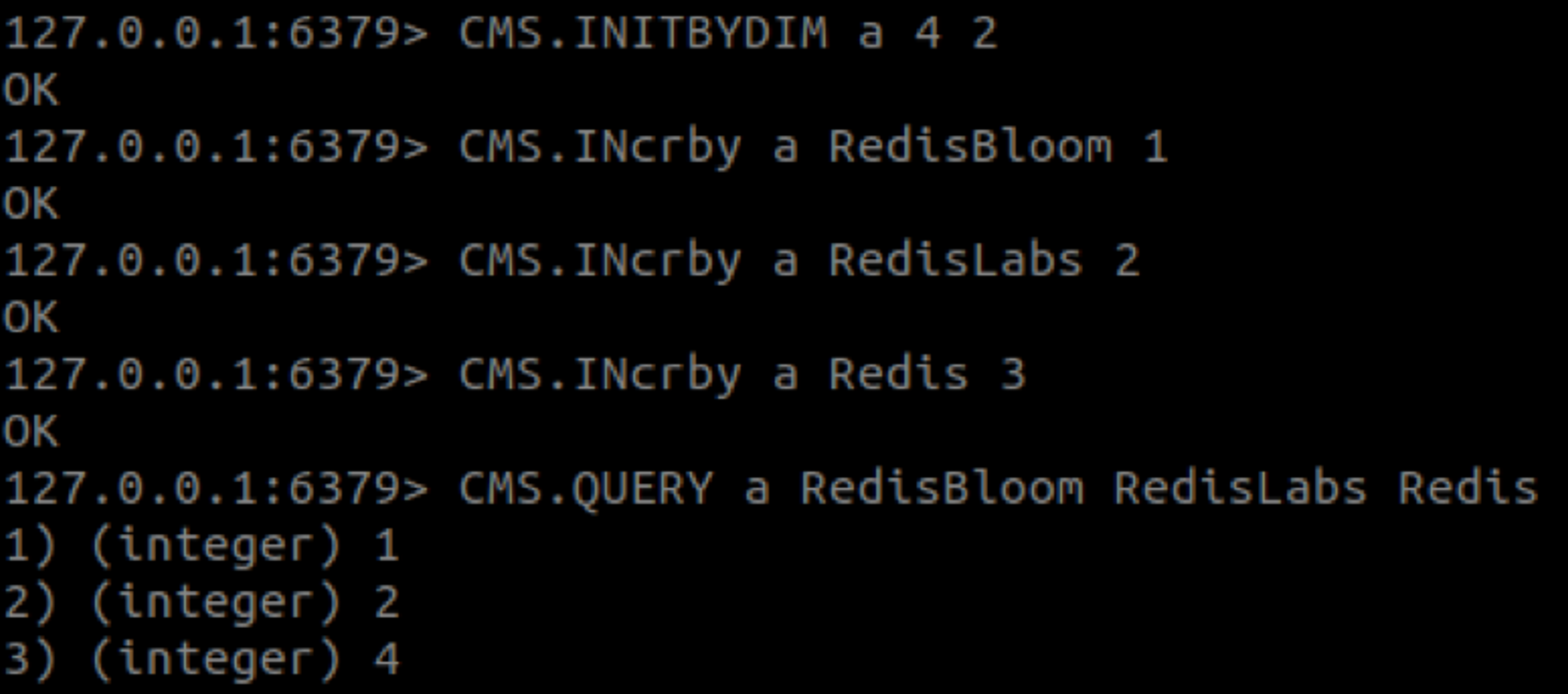
- To initialize a CM sketch data structure: INITBYDIM {key} {width} {depth} or CMS.INITBYPROB {key} {error} {probability}
- To increase the counters of an item: CMS.INCRBY {key} {item} {increment}
- To get the minimum count found in the item’s counters: CMS.QUERY {key} {item}
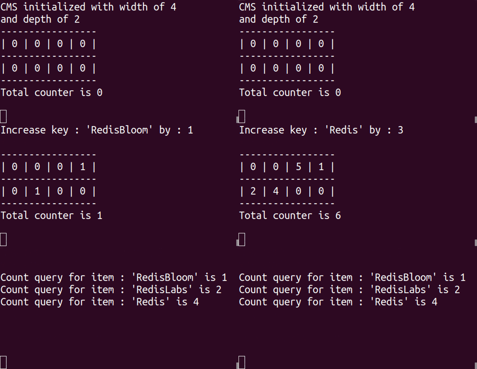
The following commands were used to create the animated example at the top of this post:

As you can see, the value of ‘Redis’ is 4 instead of 3. This behavior is expected since, in CM sketch, the count of an item is likely to be inflated.
A sketchy business
Software engineering is all about making trade-offs, and a popular approach to addressing such challenges in a cost-effective way is to forgo accuracy in favor of efficiency. This approach is exemplified by Redis’ implementation of the HyperLogLog, a data structure that’s designed to efficiently provide answers to queries about set cardinality. The HyperLogLog is a member of a family of data structures called “sketches” that, just like their real-world artistic counterparts, convey information via an approximation of their subjects.
In broad strokes, sketches are data structures (and their accompanying algorithms) that capture the nature of your data—the answers to your questions about the data, without actually storing the data itself. Formally stated, sketches are useful because they have sublinear asymptotic computational complexity, thus requiring less computing power and/or storage. But there are no free lunches and the gain in efficiency is offset by the accuracy of the answers. In many cases, however, errors are acceptable as long as they can be kept under a threshold. A good data sketch is one that readily admits its errors, and in fact, many sketches parameterize their errors (or the probability of said errors) so that they can be defined by the user.
Good sketches are efficient and have bound probability of error, but excellent sketches are those that can be computed in parallel. A parallelizable sketch is one that can be prepared independently on parts of the data and that allows combining its parts into a meaningful and consistent aggregate. Because each piece of an excellent sketch can be computed at a different location and/or time, parallelism makes it possible to apply a straightforward divide-and-conquer approach to solving scaling challenges.
A frequent problem
The aforementioned HyperLogLog is an excellent sketch but it is only suited for answering a specific type of question. Another invaluable tool is the Count Min Sketch (CMS), as described in the paper “An Improved Data Stream Summary: The Count-Min Sketch and its Applications” by G. Cormode and S. Muthukrishnan. This ingenious contraption was contrived to provide answers about the frequency of samples, a common building block in a large percentage of analytical processes.
Given enough time and resources, calculating samples’ frequency is a simple process – just keep a count of observations (times seen) for each sample (thing seen) and then divide that by the total number of observations to obtain that sample’s frequency. However, given the context of high-scale low-latency data processing, there’s never enough time or resources. Answers are to be supplied instantly as the data streams in, regardless of its scale, and the sheer size of the sampling space makes it unfeasible to keep a counter for each sample.
So instead of accurately keeping track of each sample, we can try estimating the frequency. One way of going about that is to randomly sample the observations and hope that the sample generally reflects the properties of the whole. The problem with this approach is that ensuring true randomness is a difficult task, so the success of random sampling may be limited by our selection process and/or the properties of the data itself. That is where CMS comes in with an approach so radically different, that at first, it may seem like the opposite of an excellent sketch: not only does CMS record each and every observation, each one is recorded in multiple counters!
Of course, there is a twist, and it is as clever as it is simple. The original paper (and its lighter version called “Approximating Data with the Count-Min Data Structure”) does a great job of explaining it, but I’ll try to summarize it anyway. The cleverness of CMS is in the way that it stores samples: instead of tracking each unique sample independently, it uses its hash value. The hash value of a sample is used as the index to a constant-sized (parameterized as d in the paper) array of counters. By employing several (the parameter w) different hash functions and their respective arrays, the sketch handles hash collisions found while querying the structure by picking the minimum value out of all relevant counters for the sample.
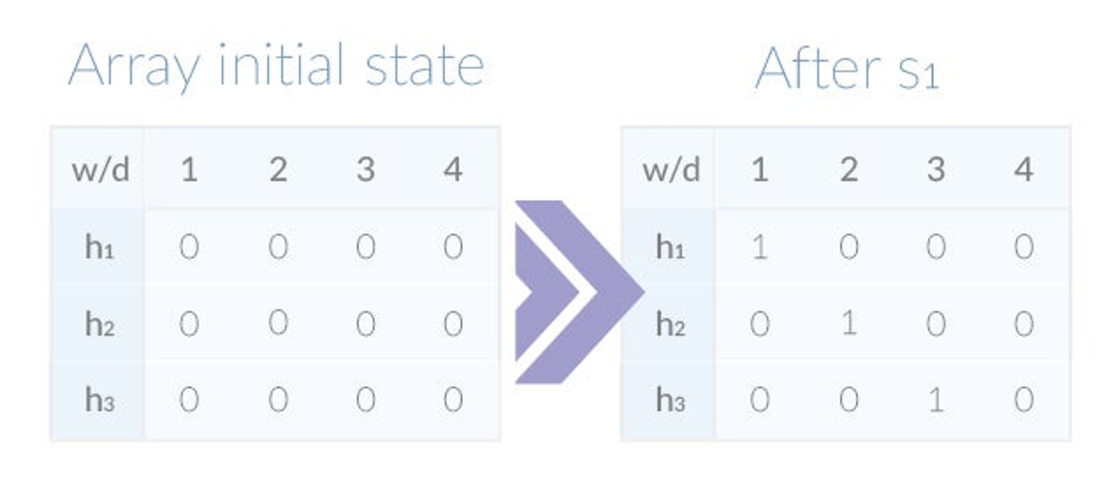
An example is called for, so let’s make a simple sketch to illustrate the data structure’s inner workings. To keep the sketch simple, we’ll use small parameter values. We’ll set w to 3, meaning we’ll use three hash functions – denoted h1, h2, and h3 respectively, and d to 4. To store the sketch’s counters we’ll use a 3×4 array with a total of 12 elements initialized to 0.
Now we can examine what happens when samples are added to the sketch. Let’s assume samples arrive one by one and that the hashes for the first sample, denoted as s1, are: h1(s1) = 1, h2(s1) = 2 and h3(s1) = 3. To record s1 in the sketch we’ll increment each hash function’s counter at the relevant index by 1. The following table shows the array’s initial and current states:

Although there’s only one sample in the sketch, we can already query it effectively. Remember that the number of observations for a sample is the minimum of all its counters, so for s1 it is obtained by:
min(array[1][h1(s1)], array[2][h2(s1)], array[3][h3(s1)]) =
min(array[1][1], array[2][2], array[3][3]) =
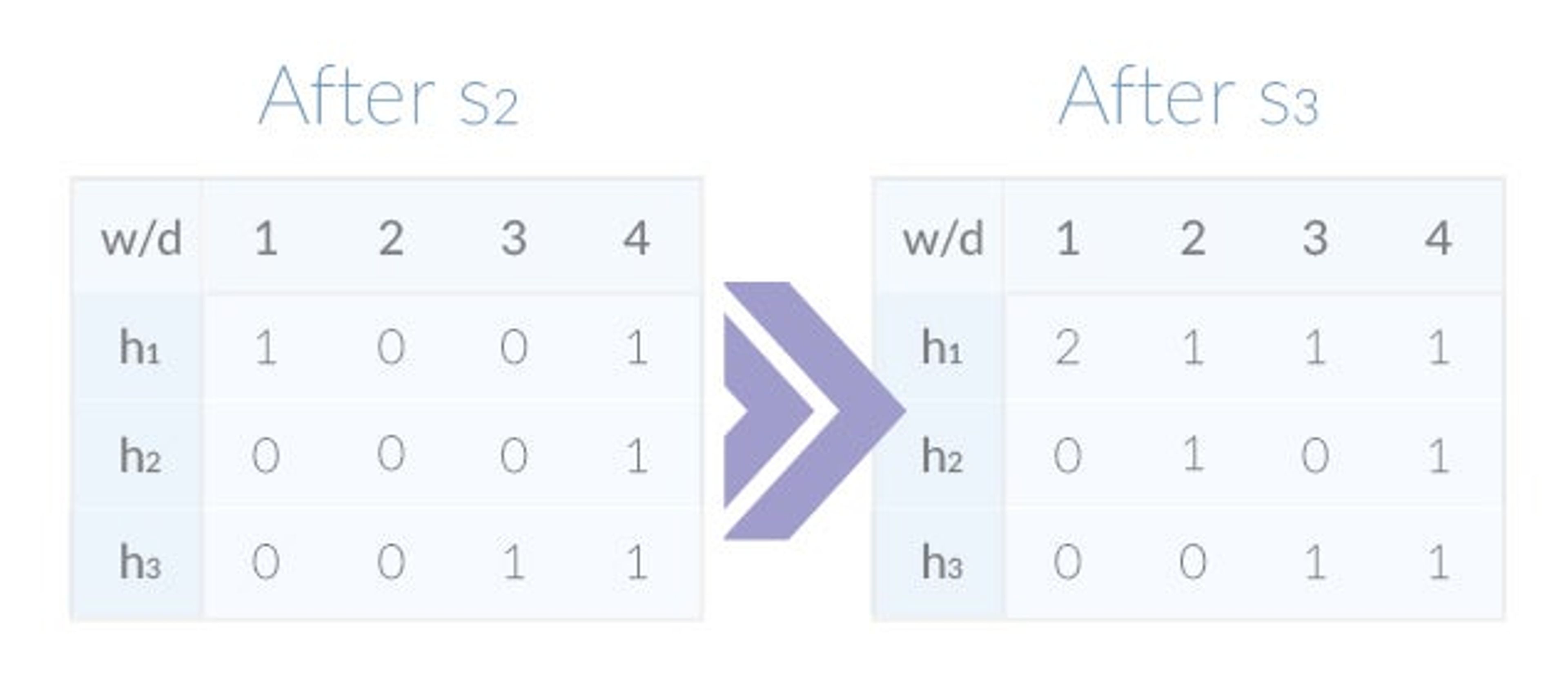
min(1,1,1) = 1The sketch also answers queries about the samples not yet added. Assuming that h1(s2) = 4, h2(s2) = 4, h3(s2) = 4, note that querying for s2 will return the result 0. Let’s continue to add s2 and s3 (h1(s3) = 1, h2(s3) = 1, h3(s3) = 1) to the sketch, yielding the following:

In our contrived example, almost all of the samples’ hashes map to unique counters, with the one exception being the collision of h1(s1) and h1(s3). Because both hashes are the same, h1‘s 1st counter now holds the value 2. Since the sketch picks the minimum of all counters, the queries for s1 and s3 still return the correct result of 1. Eventually, however, once enough collisions have occurred, the queries’ results will become less accurate.
CMS’ two parameters – w and d – determine its space/time requirements as well as the probability and maximal value of its error. A more intuitive way to initialize the sketch is to provide the error’s probability and cap, allowing it to then derive the required values for w and d. Parallelization is possible because any number of sub-sketches can be trivially merged as the sum of arrays, as long as the same parameters and hash functions are used in constructing them.
A few observations about the Count-min sketch
Count Min Sketch’s efficiency can be demonstrated by reviewing its requirements. The space complexity of CMS is the product of w, d, and the width of the counters that it uses. For example, a sketch that has a 0.01% error rate at a probability of 0.01% is created using 10 hash functions and 2000-counter arrays. Assuming the use of 16-bit counters, the overall memory requirement of the resulting sketch’s data structure clocks in at 40KB (a couple of additional bytes are needed for storing the total number of observations and a few pointers). The sketch’s other computational aspect is similarly pleasing—because hash functions are cheap to produce and compute, accessing the data structure, whether for reading or writing, is also performed in constant time.
There’s more to CMS; the sketch’s authors have also shown how it can be used for answering other similar questions. These include estimating percentiles and identifying heavy hitters (frequent items) but are out of scope for this post.
CMS is certainly an excellent sketch, but there are at least two things that prevent it from achieving perfection. My first reservation about CMS is that it can be biased, and thus overestimate the frequencies of samples with a small number of observations. CMS’ bias is well known and several improvements have been suggested. The most recent is the Count Min Log Sketch (“Approximately counting with approximate counters” from G. Pitel and G. Fouquier), which essentially replaces CMS’ linear registers with logarithmic ones to reduce the relative error and allow higher counts without increasing the width of counter registers.
While the above reservation is shared by everyone (albeit only those who grok data structures), my second reservation is exclusive to the Redis community. In order to explain, I’ll have to introduce Redis Modules.
A Redis module
Redis Modules were unveiled earlier this year at RedisConf by antirez and have literally turned our world upside-down. Nothing more or less than server-loadable dynamic libraries, Modules allow Redis users to move faster than Redis itself and go places never dreamt of before. And while this post isn’t an introduction to what Modules are or how to make them, this one is (as well as this post, and this webinar).
There are several reasons I wanted to write the Count Min Sketch Redis module, aside from its extreme usefulness. Part of it was a learning experience and part of it was an evaluation of the modules API, but mostly it was just a whole lot of fun to model a new data structure into Redis. The module provides a Redis interface for adding observations to the sketch, querying it, and merging multiple sketches into one.
The module stores the sketch’s data in a Redis String and uses direct memory access (DMA) for mapping the contents of the key to its internal data structure. I’ve yet to conduct exhaustive performance benchmarks on it, but my initial impression from testing it locally is that it is as performant as any of the core Redis commands. Like our other modules, countminsketch is open source and I encourage you to try it out and hack on it.
Before signing off, I’d like to keep my promise and share my Redis-specific reservation about CMS. The issue, which also applies to other sketches and data structures, is that CMS requires you to set it up/initialize it/create it before using it. Requiring a mandatory initialization stage, such as CMS parameters setup, breaks one of Redis’ fundamental patterns—data structures do not need to be explicitly declared before use as they can be created on-demand. To make the module seem more Redis-ish and work around that anti-pattern, the module uses default parameter values when a new sketch is implicitly implied (i.e. using the CMS.ADD command on a non-existing key) but also allows creating new empty sketches with given parameters.
Probabilistic data structures, or sketches, are amazing tools that let us keep up with the growth of big data and the shrinkage of latency budgets in an efficient and sufficiently accurate way. The two sketches mentioned in this post, and others such as the Bloom Filter and the T-digest, are quickly becoming indispensable tools in the modern data monger’s arsenal. Modules allow you to extend Redis with custom data types and commands that operate at native speed and have local access to the data. The possibilities are endless and nothing is impossible.
Want to learn more about Redis modules and how to develop them? Is there a data structure, whether probabilistic or not, that you want to discuss or add to Redis? Feel free to reach out to me with anything at my Twitter account or via email – I’m highly available 🙂
Get started with Redis today
Speak to a Redis expert and learn more about enterprise-grade Redis today.
