Time series

You can manage time series data in Redis Enterprise with Redis Stack.

Features

Query by start time and end-time
Query by labels sets
Aggregated queries (Min, Max, Avg, Sum, Range, Count, First, Last) for any time bucket
Configurable max retention period
Compaction/Roll-ups - automatically updated aggregated time series
labels index - each key has labels which allows query by labels

Memory model

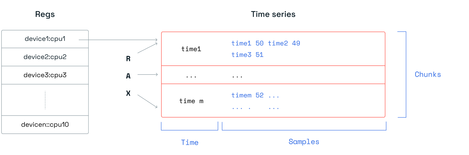
A time series is a linked list of memory chunks. Each chunk has a predefined size of samples. Each sample is a tuple of the time and the value of 128 bits, 64 bits for the timestamp and 64 bits for the value.

Time series capabilities

Redis Stack provides a new data type that uses chunks of memory of fixed size for time series samples, indexed by the same Radix Tree implementation as Redis streams. With streams, you can create a capped stream, effectively limiting the number of messages by count. For time series, you can apply a retention policy in milliseconds. This is better for time series use cases, because they are typically interested in the data during a given time window, rather than a fixed number of samples.

Downsampling/compaction

Before Downsampling	After Downsampling

If you want to keep all of your raw data points indefinitely, your data set grows linearly over time. However, if your use case allows you to have less fine-grained data further back in time, downsampling can be applied. This allows you to keep fewer historical data points by aggregating raw data for a given time window using a given aggregation function. Time series support downsampling with the following aggregations: avg, sum, min, max, range, count, first, and last.

Secondary indexing

When using Redis’ core data structures, you can only retrieve a time series by knowing the exact key holding the time series. Unfortunately, for many time series use cases (such as root cause analysis or monitoring), your application won’t know the exact key it’s looking for. These use cases typically want to query a set of time series that relate to each other in a couple of dimensions to extract the insight you need. You could create your own secondary index with core Redis data structures to help with this, but it would come with a high development cost and require you to manage edge cases to make sure the index is correct.

Redis does this indexing for you based on field value pairs called labels. You can add labels to each time series and use them to filter at query time.

Here’s an example of creating a time series with two labels (sensor_id and area_id are the fields with values 2 and 32 respectively) and a retention window of 60,000 milliseconds:

    TS.CREATE temperature RETENTION 60000 LABELS sensor_id 2 area_id 32

Aggregation at read time

When you need to query a time series, it’s cumbersome to stream all raw data points if you’re only interested in, say, an average over a given time interval. Time series only transfer the minimum required data to ensure lowest latency.

Here's an example of aggregation over time buckets of 5,000 milliseconds:

    127.0.0.1:12543> TS.RANGE temperature:3:32 1548149180000 1548149210000 AGGREGATION avg 5000
    1) 1) (integer) 1548149180000
       2) "26.199999999999999"
    2) 1) (integer) 1548149185000
       2) "27.399999999999999"
    3) 1) (integer) 1548149190000
       2) "24.800000000000001"
    4) 1) (integer) 1548149195000
       2) "23.199999999999999"
    5) 1) (integer) 1548149200000
       2) "25.199999999999999"
    6) 1) (integer) 1548149205000
       2) "28"
    7) 1) (integer) 1548149210000
       2) "20"

Integrations

Redis Stack comes with several integrations into existing time series tools. One such integration is our RedisTimeSeries adapter for Prometheus, which keeps all your monitoring metrics inside time series while leveraging the entire Prometheus ecosystem.

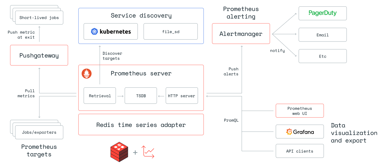
Furthermore, we also created direct integrations for Grafana. This repository contains a docker-compose setup of RedisTimeSeries, its remote write adaptor, Prometheus and Grafana. It also comes with a set of data generators and pre-built Grafana dashboards.

Time series modeling approaches with Redis

Data modeling approaches

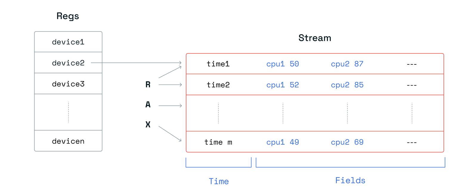
Redis streams allow you to add several field value pairs in a message for a given timestamp. For each device, we collected 10 metrics that were modeled as 10 separate fields in a single stream message.

For sorted sets, we modeled the data in two different ways. For “Sorted set per device”, we concatenated the metrics and separated them out by colons, e.g. “<timestamp>:<metric1>:<metric2>: … :<metric10>”.

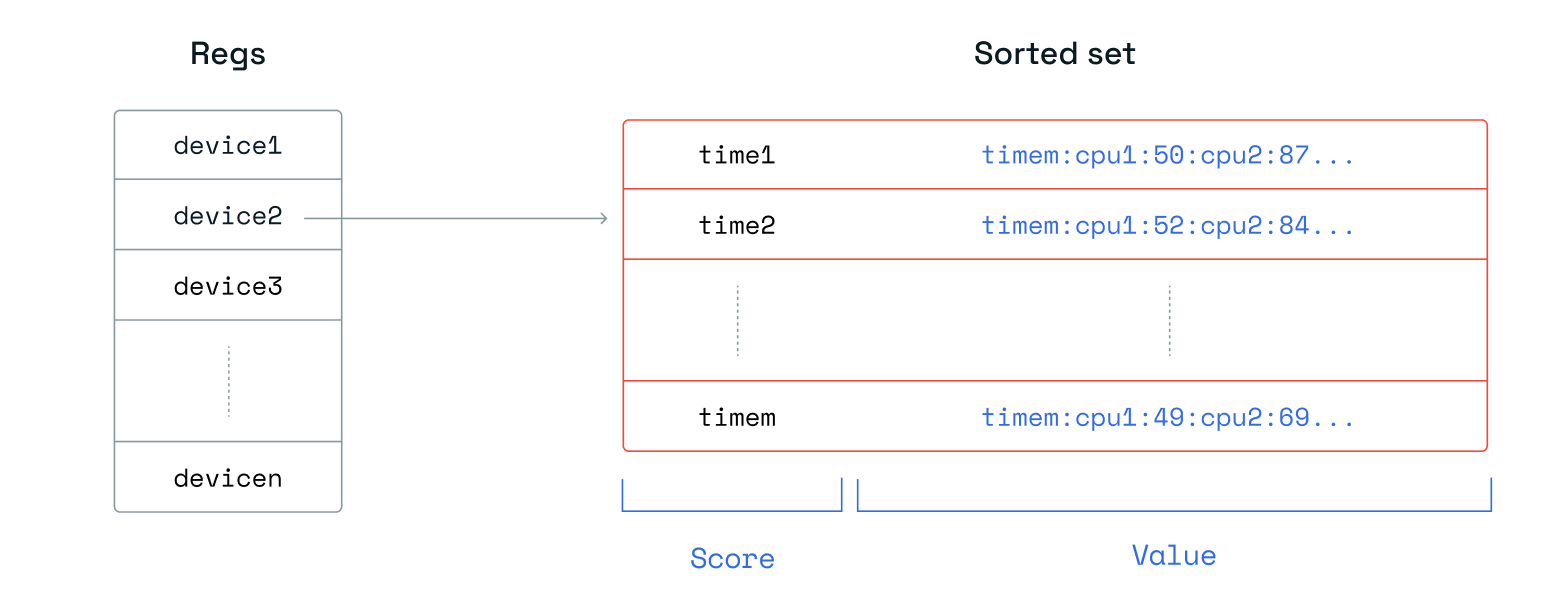
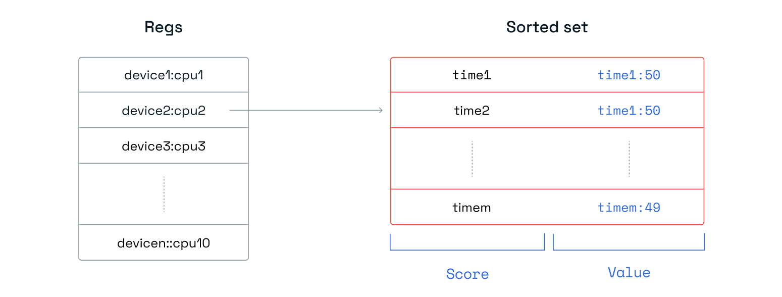
Of course, this consumes less memory but needs more CPU cycles to get the correct metric at read time. It also implies that changing the number of metrics per device isn’t straightforward, which is why we also benchmarked a second sorted set approach. In “Sorted set per metric,” we kept each metric in its own sorted set and had 10 sorted sets per device. We logged values in the format “<timestamp>:<metric>”.

Another alternative approach would be to normalize the data by creating a hash with a unique key to track all measurements for a given device for a given timestamp. This key would then be the value in the sorted set. However, having to access many hashes to read a time series would come at a huge cost during read time, so we abandoned this path.

Each time series holds a single metric. We chose this design to maintain the Redis principle that a larger number of small keys is better than a fewer number of large keys.

Our benchmark did not utilize the out-of-the-box secondary indexing capabilities of time series. Redis keeps a partial secondary index in each shard, and since the index inherits the same hash-slot of the key it indexes, it is always hosted on the same shard. This approach would make the setup for native data structures even more complex to model, so for the sake of simplicity, we decided not to include it in our benchmarks. Additionally, while Redis Enterprise can use the proxy to fan out requests for commands like TS.MGET and TS.MRANGE to all the shards and aggregate the results, we chose not to exploit this advantage in the benchmark either.

Data ingestion

For the data ingestion part of our benchmark, we compared the four approaches by measuring how many devices’ data we could ingest per second. Our client side had 8 worker threads with 50 connections each, and a pipeline of 50 commands per request.

Ingestion details of each approach:

	Redis streams	Time series	Sorted set per device	Sorted set per metric
Command	XADD	TS.MADD	ZADD	ZADD
Pipeline	50	50	50	50
Metrics per request	5000	5000	5000	500
# keys	4000	40000	4000	40000

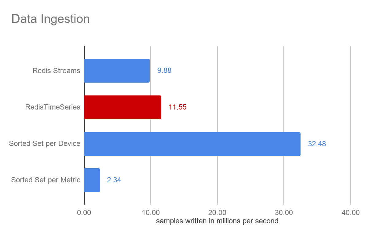
All our ingestion operations were executed at sub-millisecond latency. Although both used the same Rax data structure, the time series approach has slightly higher throughput than Redis streams.

Each approach yields different results, which shows the value of prototyping against specific use cases. As we see on query performance, the sorted set per device comes with improved write throughput but at the expense of query performance. It’s a trade off between ingestion, query performance, and flexibility (remember the earlier data modeling remark).

Read performance

The read query we used in this benchmark queried a single time series and aggregated it in one-hour time buckets by keeping the maximum observed CPU percentage in each bucket. The time range we considered in the query was exactly one hour, so a single maximum value was returned. For time series, this is out of the box functionality.

    127.0.0.1:12543> TS.RANGE cpu_usage_user{1340993056} 1451606390000 1451609990000 AGGREGATION max 3600000

For the Redis streams and sorted sets approaches, we created the following LUA scripts. The client once again had 8 threads and 50 connections each. Since we executed the same query, only a single shard was hit, and in all four cases this shard maxed out at 100% CPU.

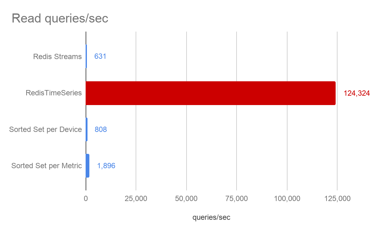
This is where you can see the real power of having dedicated data structure for a given use case with a toolbox that runs alongside it. Using time series exceeds all other approaches and is the only one to achieve sub-millisecond response times.

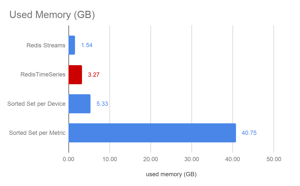
Memory utilization

For both the Redis streams and sorted set approaches, the samples were stored as strings, while time series stored them as doubles. In this specific data set, we chose a CPU measurement with rounded integer values between 0-100, which thus consumes two bytes of memory as a string. With time series, each metric had 64-bit precision.

Time series can dramatically reduce the memory consumption when compared against both sorted set approaches. Given the unbounded nature of time series data, this is typically a critical criteria to evaluate - the overall data set size that needs to be retained in memory. Redis streams reduces the memory consumption further but would be equal or higher than time series when more digits for a higher precision would be required.