Blog
An Introduction to Redis-ML. Part One
Despite widespread interest in machine learning (ML), using it effectively in a real-time environment is a complex problem that hasn’t been given enough attention by framework developers. Nearly every language has a framework to implement the “learning” part of machine learning, but very few frameworks support the “predict” side of machine learning.
Once you’ve trained an ML model, how can you build a real-time application based on that model? With many toolkits, you have to build your own application. We are just starting to see frameworks focused on the prediction side of machine learning.
An earlier post provided an overview of the features available in the Redis-ML module, so in this post, we’re going to dive deeper into machine learning – explain some of the techniques in an accessible way and show how you can augment a machine learning pipeline with Redis. As an example, we will walk through the code for a sample program for predicting median housing prices from various features of a neighborhood.
The sample code in this post is written in Python 3 using a variety of freely available packages for machine learning. You will need to install the following packages, using pip3 or your preferred package manager, to run the samples:
- scikit-learn (0.18.2)
- numpy (1.13.1)
- scipy (0.19.1)
- redis (2.10.5)
You will also need a Redis 4.0.0 instance and the Redis-ML module. Shay Nativ, the developer behind the Redis-ML module, created a Docker container with Redis 4.0.0 and the Redis-ML module preloaded. To use that container in conjunction with the code in this post, launch the container using the command:
Docker will automatically download and run the container, mapping the default Redis port (6379) from the container to your computer.
To build our housing price predictor, we will use a machine learning technique known as linear regression.
Linear regression was part of the statistician’s toolbox long before algorithmic machine learning was invented. With linear regression, we attempt to predict a result (sometimes called the dependent value) from one or more known quantities (explanatory variables). For linear regression to work, we must be able to accurately estimate our results with a straight line.
In the graph above, taken from the Wikipedia article on Linear Regression, we can see how our data points cluster around an idealized line. This data set is a good candidate for linear regression. In practice, linear regression is used to model a variety of real-world problems where a linear relationship from observations can accurately predict a result, such as the price of a house based on square footage, or college GPA from high school GPA and SAT scores.
From algebra we know that a line is represented by an equation of the form y = b + ax, so to “learn” a model of this form, we need to apply an algorithm to discover the parameters of the line – the slope and intercept. Nothing incredibly fancy, in fact prior to algorithmic machine learning, most statistician would “fit” these models by hand. These days, it’s far more common to use a computer to find the line’s parameters and a variety of tool kits (TensorFlow, Scikit, Apache Spark) are available to solve a linear regression problem. The important thing to remember is that once we’ve learned a linear regression model, we have a mathematical formula for predicting results that could be implemented by any system.
Let’s work through an example of performing a linear regression and discovering the model parameters using the popular Python scikit-learn package and the Boston Housing dataset.
The Boston Housing Dataset is a classic data set used in teaching statistics and machine learning. The dataset predicts the median housing price for a neighborhood in the Boston area using neighborhood features like the average number of rooms in a house, the distance from main Boston employment centers, or crime rate. To make it easier to visualize the linear regression process, we’re going to work with a single feature of the data, the average rooms per dwelling (RM) column.

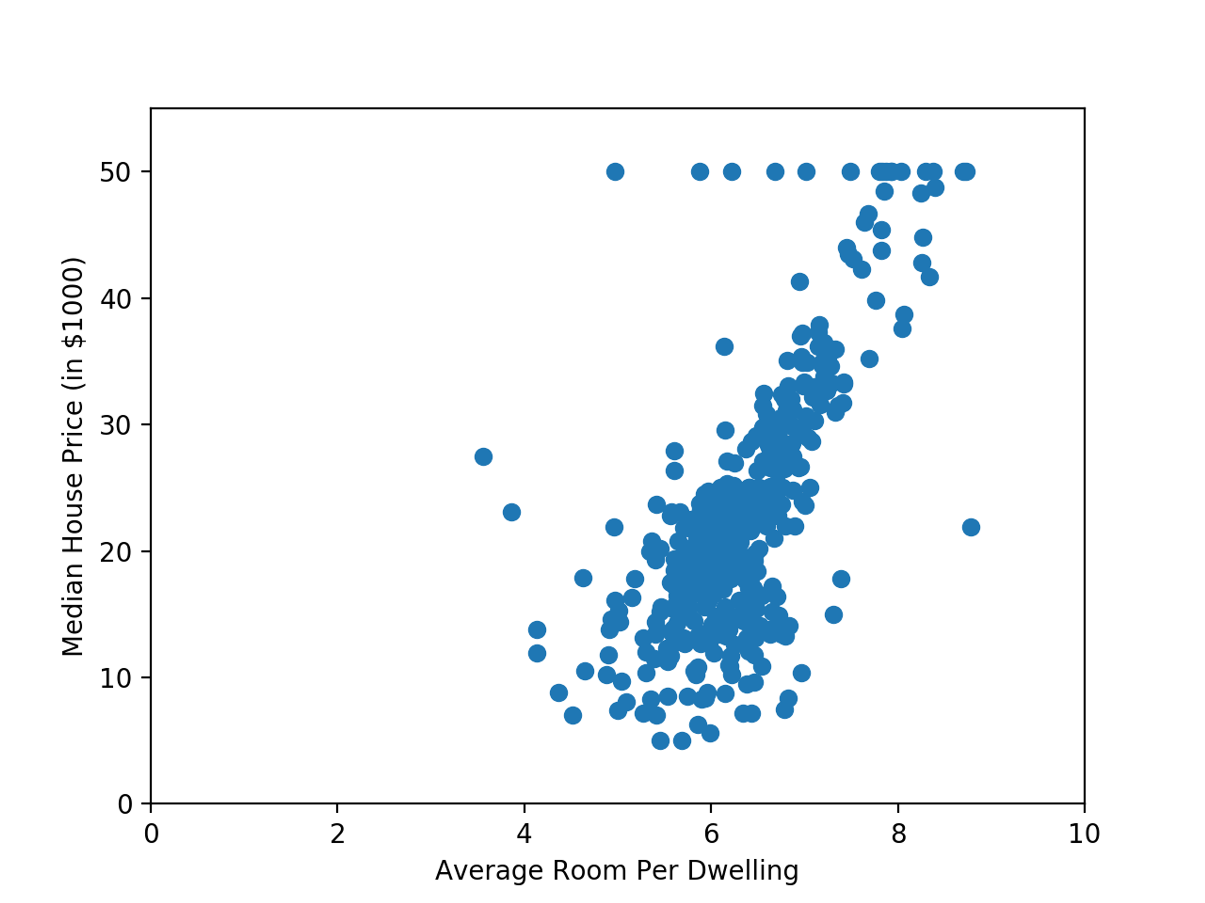
The Boston Housing Dataset is provided as part of the scikit-learning package, so, let’s start by plotting our data to visualize the relationship between room count (RM) and median price (MEDV):

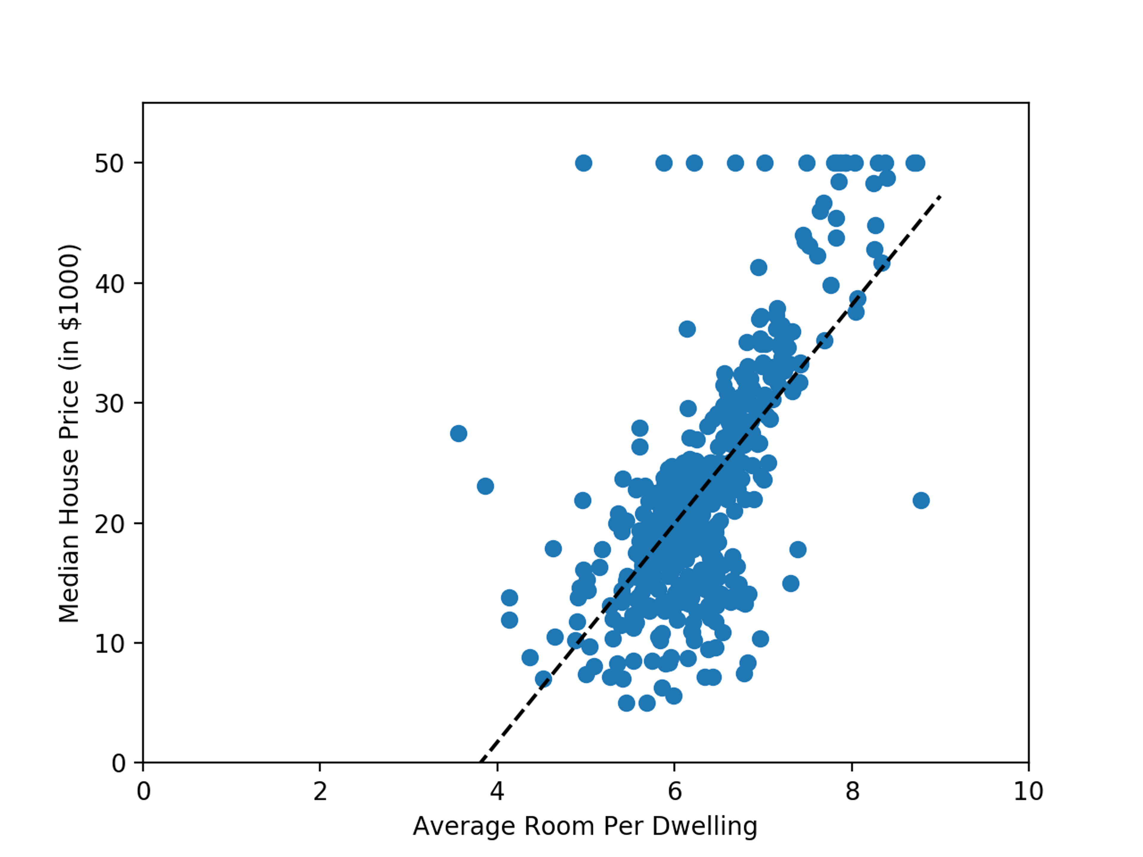
While not a perfect line, we can see a pretty strong linear relationship between the average number of rooms and the median house price in a neighborhood. We can even draw an idealized representation of the relationship and see how the data points cluster around it.
The following code demonstrates how to load the Boston Housing dataset using scikit. The Boston Housing dataset consists of twelve different features used to predict housing prices, so after loading the dataset, we extract data from the fifth column (the RM column) from the data for our sample.
Now we split our data into two sets, a training set and a test set. For our example, we create our training set from the first 400 samples and the test set from the remaining 106 samples.
This method of splitting ensure ensures we always run with the same sets for reproducible results.
Now that we’ve constructed our training and test sets, we can use the LinearRegression model supplied by scikit to fit a line to our data:
After running our code, we find that scikit has fit a line to our data with a coefficient of 9.40550212 and an intercept of -35.26094818316348.
Now that we have these parameters, we can implement a linear model to predict housing prices in the Boston area based on the average number of rooms in a house in a neighborhood of interest. Now that I have this model, how can I build an application to make real-time predictions and use the functionality an app or a website?
The Scikit package provides a predict function to evaluate a trained model, but using a function within an application requires implementing a host of other services to make it fast and reliable. This is where Redis can augment your machine learning systems.
The Redis-ML module takes advantage of the new Modules API to add a standard linear regression as a native datatype. The module can create linear regressions as well as use them to predict values.
To add a linear regression to Redis, you need to use the ML.LINREG.SET command to add a linear regression to the database. The ML.LINGREG.SET command has the following form:
By convention, all of the commands in the Redis-ML module begin with the module’s identifier, ML. All linear regression commands are prefixed with LINGREG.
To setup Redis to be a predictive engine for Boston housing prices using the line we fit in scikit, we need to first load the Redis-ML module using the loadmodule directive.
Then we set a key to represent our linear regression using the constants from scikit by executing the ML.LINGREG.SET command. Remember that the intercept is the first value supplied and the coefficients are provided in feature order. From our scikit code to fit a regression line to the housing data, we determined our line had a coefficient of 9.40550212 for the RM variable and an intercept of -35.26094818316348. We can use the ML.LINGREG.SET command to set a Redis key to compute this linear relationship:
Once our boston_house_price:rm-only key is created, we can repeatedly predict the median house price in a neighborhood by using the ML.LINGREG.PREDICT command. To predict the median house price in a neighborhood that averages 6.2 rooms per house we would run the command:
Redis predicts a median house price of $23,053 (remember our housing prices are in thousands) for this neighborhood.
It’s helpful to understand how to work with the ML.LINREG commands from the redis-cli, but it is far more likely we would be doing this from an application. We can extend our Python code which fits the regression line to automatically create the boston_house_price:rm-only key in Redis. Once we’ve created the key in Redis, we implement a test that generates predictions from Redis using our test data.
We can also generate scikit’s predictions for the same set of data using the predict routine:

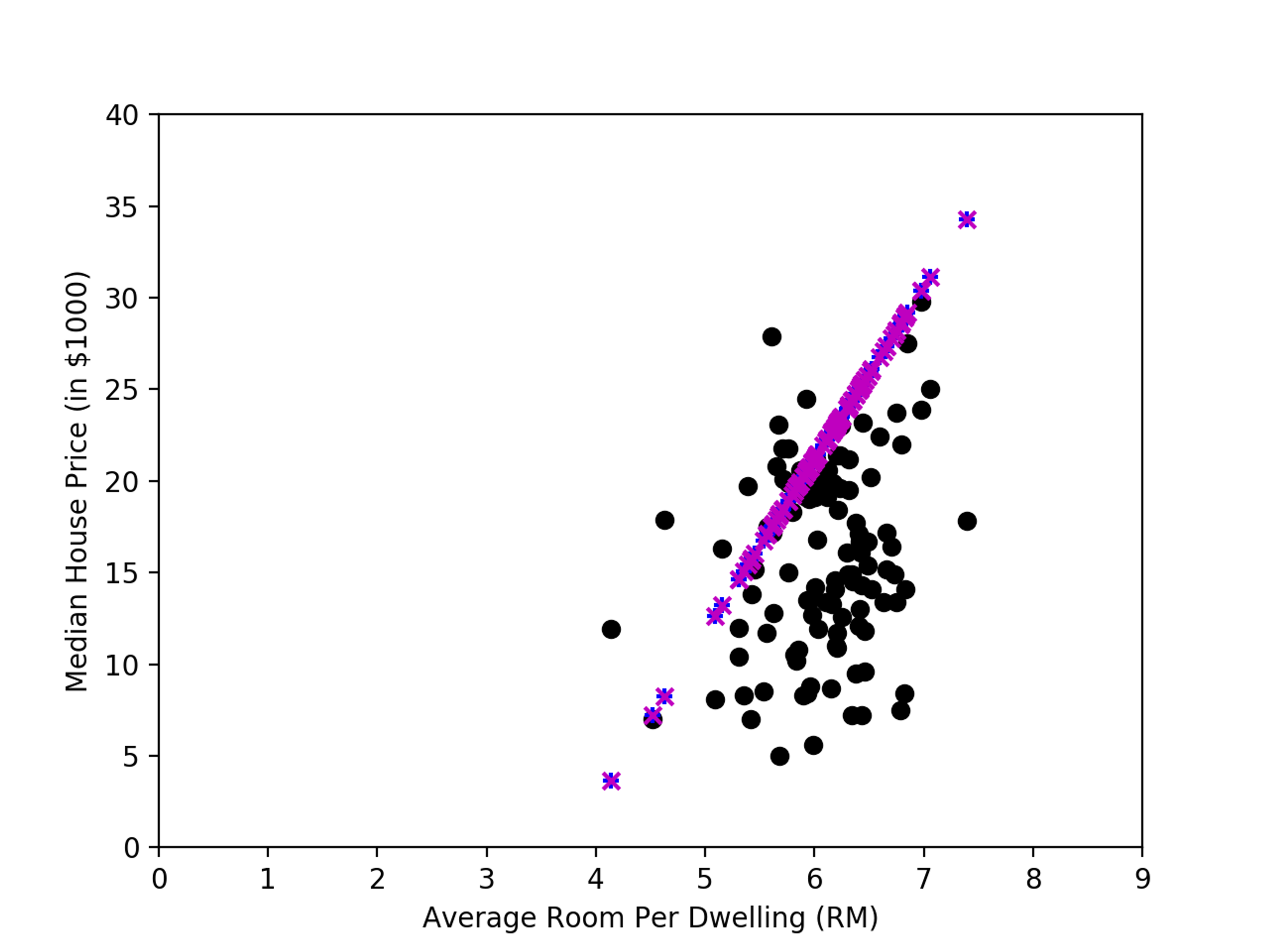
For comparison, we’ve plotted the results. In the graph below, the black circles represent the actual prices for the test data in our dataset. The blue markers (+) represent the values predicted by Scikit and the magenta markers (x) represent the values predicted by Redis.
As you can see the Redis and scikit make the same predictions for median house price given the average number of rooms. While linear regression may not correctly predict the exact price of every data point, it provides a useful means of estimating an unknown price based on some observable features of a neighborhood.
In this post, we dug deeper into the linear regression feature of the Redis-ML. We looked at how to use the popular scikit Python package to fit a linear regression line to some housing data and then create a housing price prediction engine using Redis 4.0.0 and the Redis-ML module.
In the next part of the series we will look at how Redis-ML can be used to implement an engine for classification, another kind of machine learning problem that attempts to determine the class of unknown data from previous examples.
Get started with Redis today
Speak to a Redis expert and learn more about enterprise-grade Redis today.
