“Simplicity is the ultimate sophistication”—Leonardo da Vinci

“Most information is irrelevant and most effort is wasted, but only the expert knows what to ignore”—James Clear, Atomic Habits

You have a fancy data pipeline with lots of different systems. It looks very sophisticated on the surface, but it’s actually a complex mess under the hood. It might need a lot of plumbing work to connect different pieces, it might need constant monitoring, it might require a large team with unique expertise to run, debug and manage it. Not to mention, the more systems you use, the more places you are duplicating your data and the more chances of it going out-of-sync or stale. Furthermore, since each of these subsystems are developed independently by different companies, their upgrades or bug fixes might break your pipeline and your data layer. 

If you aren’t careful, you may end up with the following situation as depicted in the three-minute video below. I highly recommend you watch it before you proceed.

Complexity arises because even though each system might appear simple on the surface, they actually bring the following variables into your pipeline and can add a ton of complexity:

1. Protocol—how does the system transport the data? (HTTP, TCP, REST, GraphQL, FTP, JDBC)
2. Data format—what format does the system support? (Binary, CSV, JSON, Avro)
3. Data schema and evolution—how is the data stored? (tables, Streams, graphs, documents)
4. SDKs and APIs—does the system provide the necessary SDKs and APIs?
5. ACID and BASE—does it provide ACID or BASE consistency?
6. Migration—does the system provide an easy way to migrate all the data into or away from the system?
7. Durability—what guarantees does the system have around durability?
8. ility—what guarantees does the system have around availability? (99.9%, 99.999%)
9. Scalability—how does it scale?
10. Security—how secure is the system?
11. Performance—how fast is the system in processing the data?
12. Hosting options—is it hosted or on-premise only or a mix?
13. Clouds—does it work on my cloud, region, etc.?
14. Additional systems—does it need an additional system? (e.g. Zookeeper for Kafka)

The variables such as the data format, schema and protocol add up to what’s called the “transformation overhead.” Other variables like performance, durability and scalability add up to what’s called the “pipeline overhead.” Put together, these classifications contribute to what’s known as the “impedance mismatch.” If we can measure that, we can calculate the complexity and use that to simplify our system. We’ll get to that in a bit.

Now, you might argue that your system, although it might appear complex, is actually the simplest system for your needs. But how can you prove that?

In other words, how do you really measure and tell if your data layer is truly simple or complex? And secondly, how can you estimate if your system will remain simple as you add more features? That is, if you add more features in your roadmap, do you also need to add more systems?

That’s where the “impedance mismatch test,” comes in. But let’s first look into what an impedance mismatch is and then we’ll get into the test itself.

What is Impedance Mismatch?

The term originated in electrical engineering to explain the mismatch in electrical impedance, resulting in the loss of energy when energy is being transferred from point A to point B.

Simply said, it means that what you have doesn’t match what you need. To use it, you take what you currently have, transform it into what you need, and then use it. Hence there is a mismatch and an overhead associated with fixing the mismatch. 

In our case, you have the data in some form or some quantity, and you need to transform it before we can use it. The transformation might happen multiple times and might even use multiple systems in between.

In the database world, the impedance mismatch happens for two reasons:

1. Transformational overhead: The way the system processes or stores the data differs from what the data actually looks like, or how you think about it. For example: In your server, you have the flexibility to store the data in numerous data structures, such as collections, streams, Lists, Sets, Arrays, and so on. It helps you naturally model your data. However, you need to then map this data into tables in RDBMS or JSON document stores, in order to store them. Then do the opposite for reading the data. Note that the specific mismatch between object-oriented language models and relational table models is known as, “Object-relational impedance mismatch.”
2. Pipeline overhead: The amount of data and the type of data you process in the server differs from the amount of data your database can handle. For example: if you are processing millions of events that are coming from mobile devices, your typical RDBMS or document store might not be able to store it, or provide APIs to easily aggregate or calculate those events. So you need special stream-processing systems, such as Kafka or Redis Streams, to process it and also, maybe a data warehouse to store it.

The Impedance Mismatch Test

The goal of the test is to measure the complexity of the overall platform and whether the complexity grows or shrinks as you add more features in the future. 

The way the test works is to simply calculate the “transformational overhead” and the “pipeline overhead,” using an “Impedance Mismatch Score” (IMS). This will tell you if your system is already complex relative to other systems, and also if that complexity grows over time as you add more features.

Here is the formula to calculate IMS:

The formula simply adds both types of overheads and then divides them by the number of features. This way, you’ll get the total overhead/feature (i.e. complexity score). 

To understand this better, let’s compare four different simple data pipelines and calculate their scores. And secondly, let’s also imagine we are building a simple app in two phases, so that we can see how the IMS score changes as we add more features over time.

Phase 1: Building a real-time dashboard

Say you are getting millions of button-click events from mobile devices and you need an alert if there is any drop or spike. Additionally, you are considering this entire thing as a feature of your larger application. 

Case 1: Say you just used a RDBMS to store these events, although the tables might not fit.

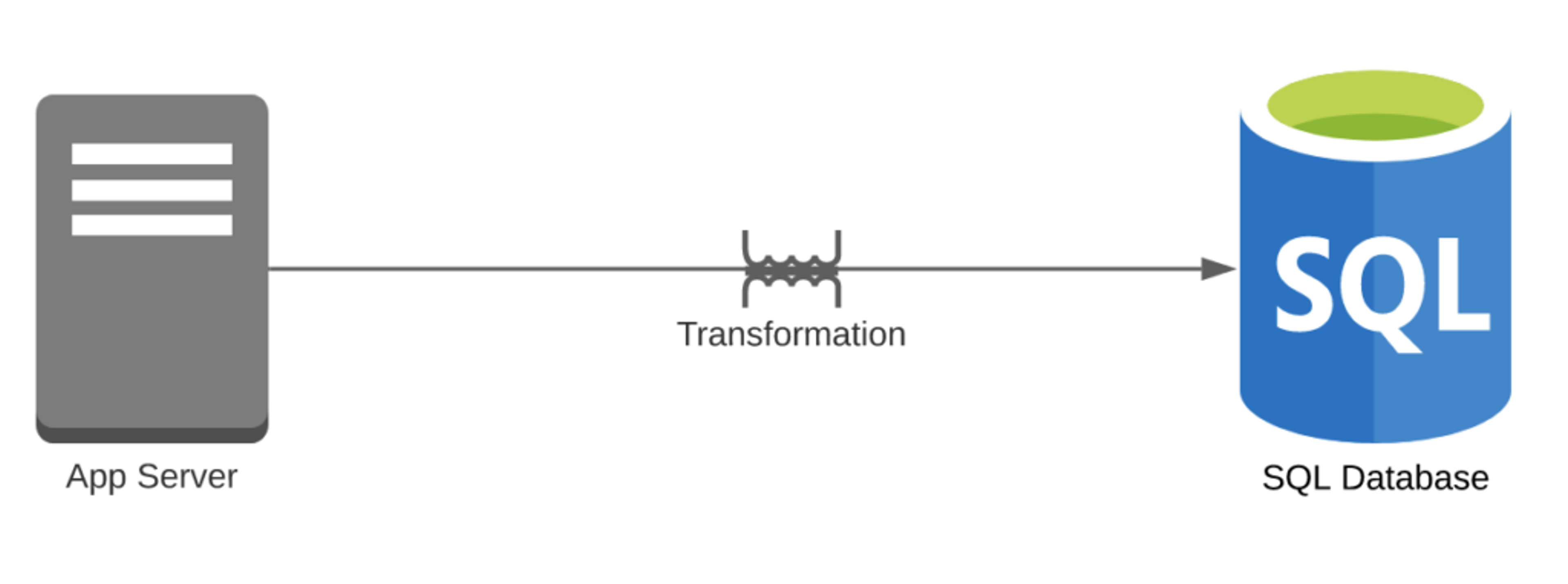
1. Transformational overhead = 1
   1. You need to transform event streams into tables.
2. Pipeline overhead = 1
   1. You have a single DB in your pipeline.
3. Number of features = 1

Case 2: Say you used Kafka to process these events and then stored them into the RDBMS.

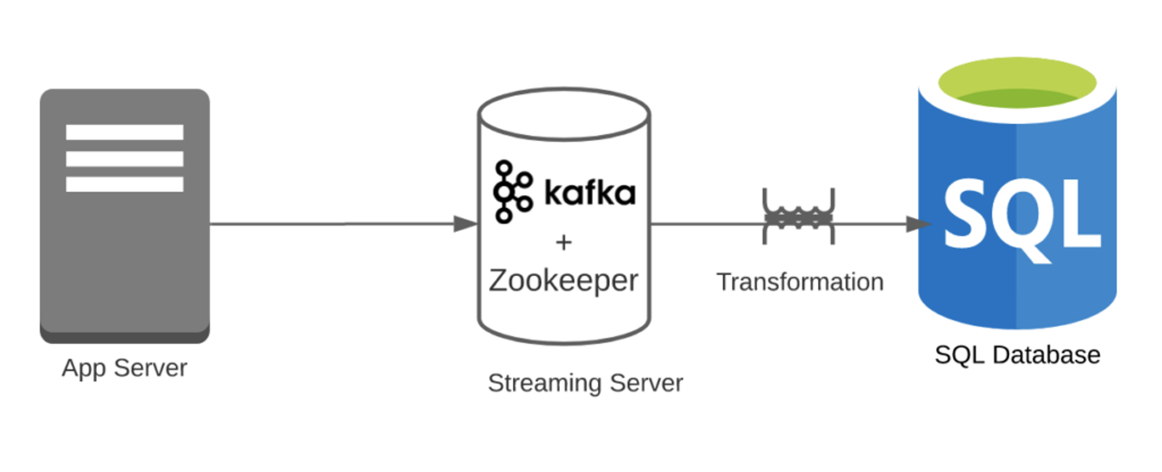
1. Transformational overhead = 1
   1. Kafka can easily handle click streams; however, Kafka to RDBMS is an overhead.
2. Pipeline overhead = 2
   1. You have two systems (RDBMS and Kafka). Note that we are ignoring Zookeeper.
3. Number of features = 1

Case 3: Say you used Kafka to process these events and then stored them into KsqlDB.

1. Transformational overhead = 0
   1. Kafka can easily handle click streams
2. Pipeline overhead = 1
   1. You have just one system ( Kafka + KSqlDB). Note that we are ignoring Zookeeper.
3. Number of features = 1

Case 4: Say you used Redis Streams to process these events and then stored them into RedisTimeseries (both are part of Redis and work natively with Redis).

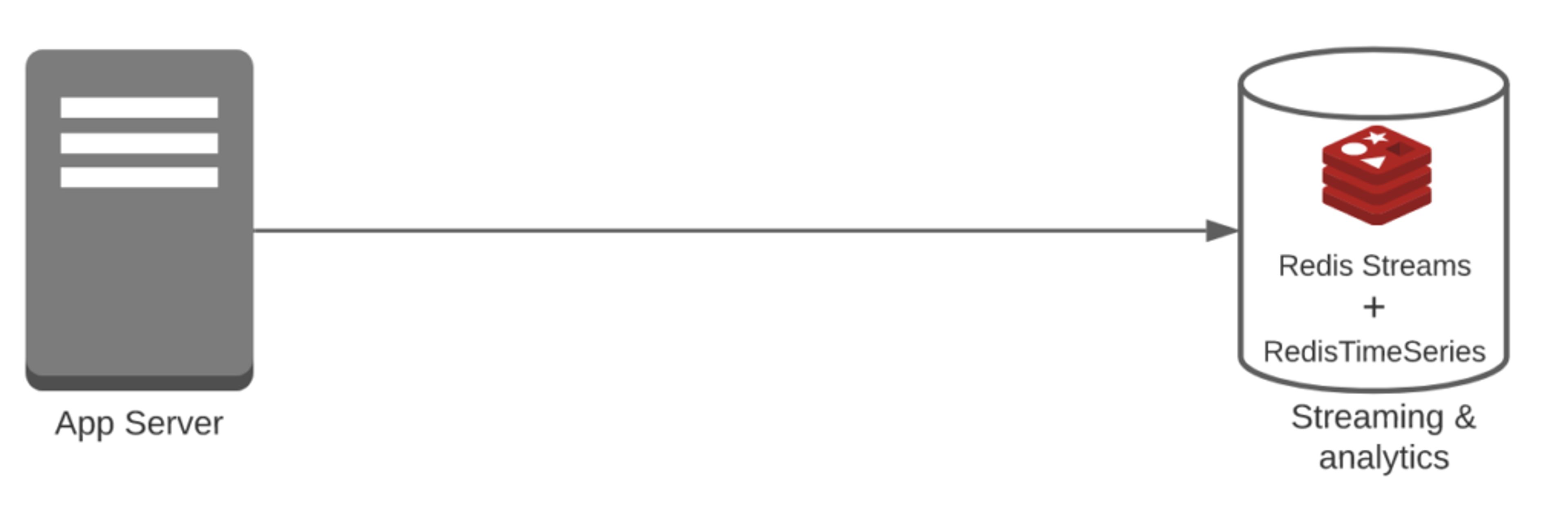
1. Transformational overhead = 0
   1. Redis Streams can easily handle click streams
2. Pipeline overhead = 1
   1. You have just one system (Redis Streams + RedisTimeSeries)
3. Number of features = 1

Conclusion after Phase 1: 

We compared four systems in this example and found out that “Case 3” or “Case 4” are the simplest with an IMS of 1. At this point, they both are the same, but will they remain the same when we add more features?

Let’s add more features to our system and see how IMS holds up.

Phase 2: Building a Real-Time Dashboard With IP-Whitelisting

Let’s say you are building the same app but want to make sure they come from only white-listed IP addresses. Now you are adding a new feature.

Case 1: Say you just used RDBMS to store these events, although the tables might not fit and they used Redis or MemCached for IP-whitelisting. 

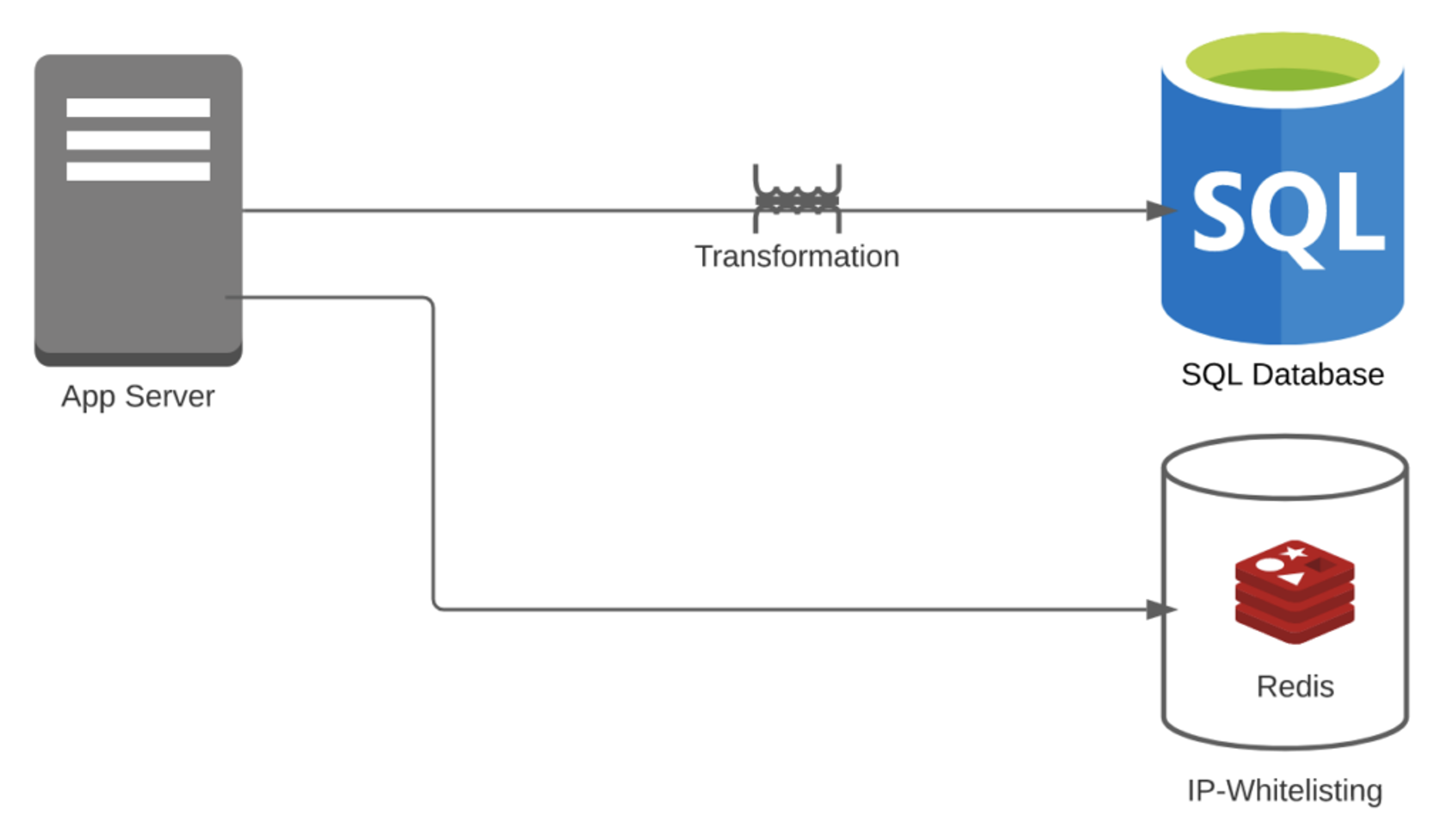
1. Transformational overhead = 1
   1. For IP-whitelisting, you don’t need any transformation. However, you need to transform event streams into tables
2. Pipeline overhead = 2
   1. You have Redis + RDBMS
3. Number of features = 2

Case 2: Say you are using Redis + Kafka + RDBMS. 

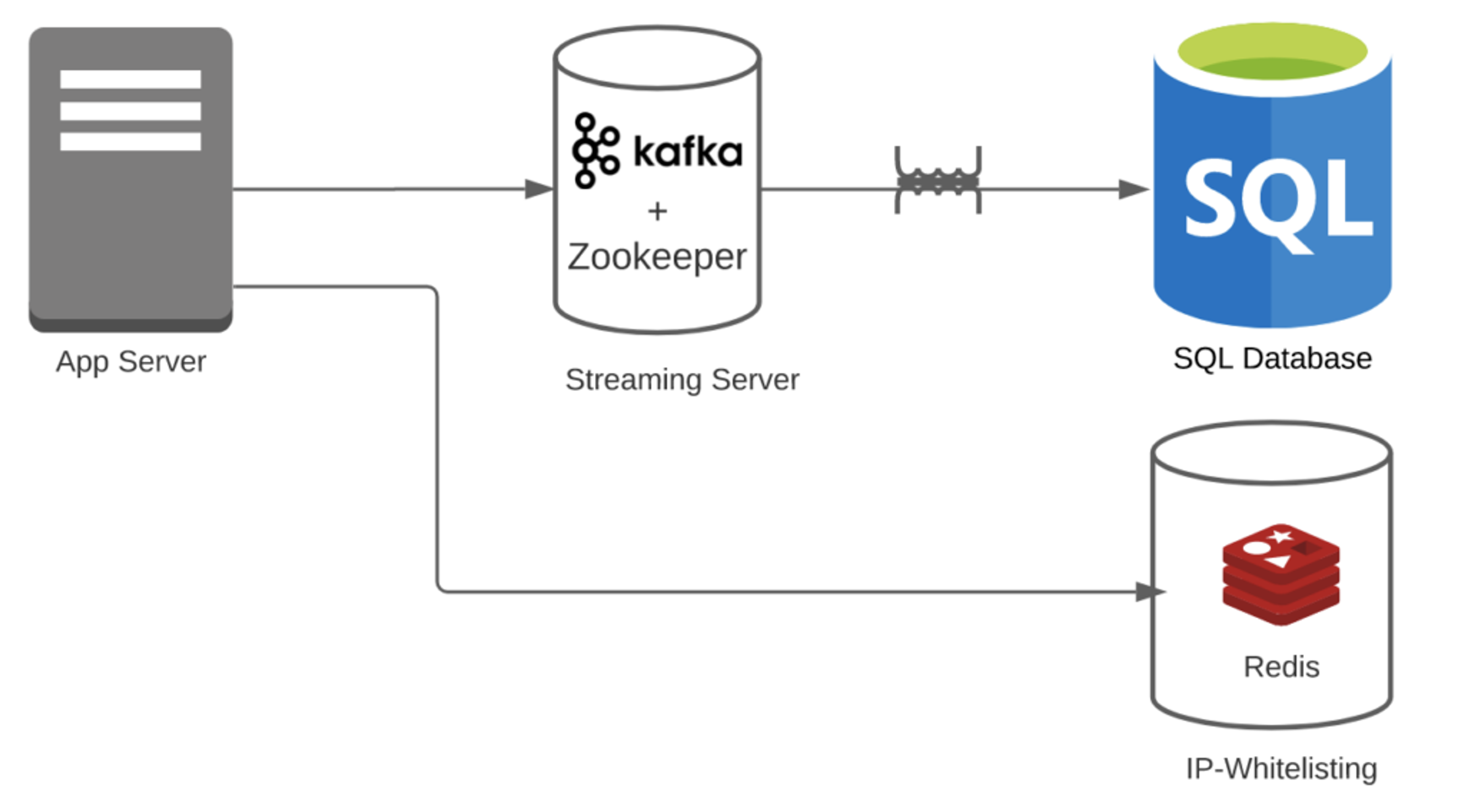
1. Transformational overhead = 1
   1. For IP-whitelisting, you don’t need any transformation. Also, Kafka can easily handle streams.
2. Pipeline overhead = 3
   1. You have Redis + Kafka + RDBMS. Note: We are ignoring that Kafka also needs Zookeeper. If you add that, the number will go down further.
3. Number of features = 2

Case 3: Say you are using Redis + Kafka + KsqlDB. 

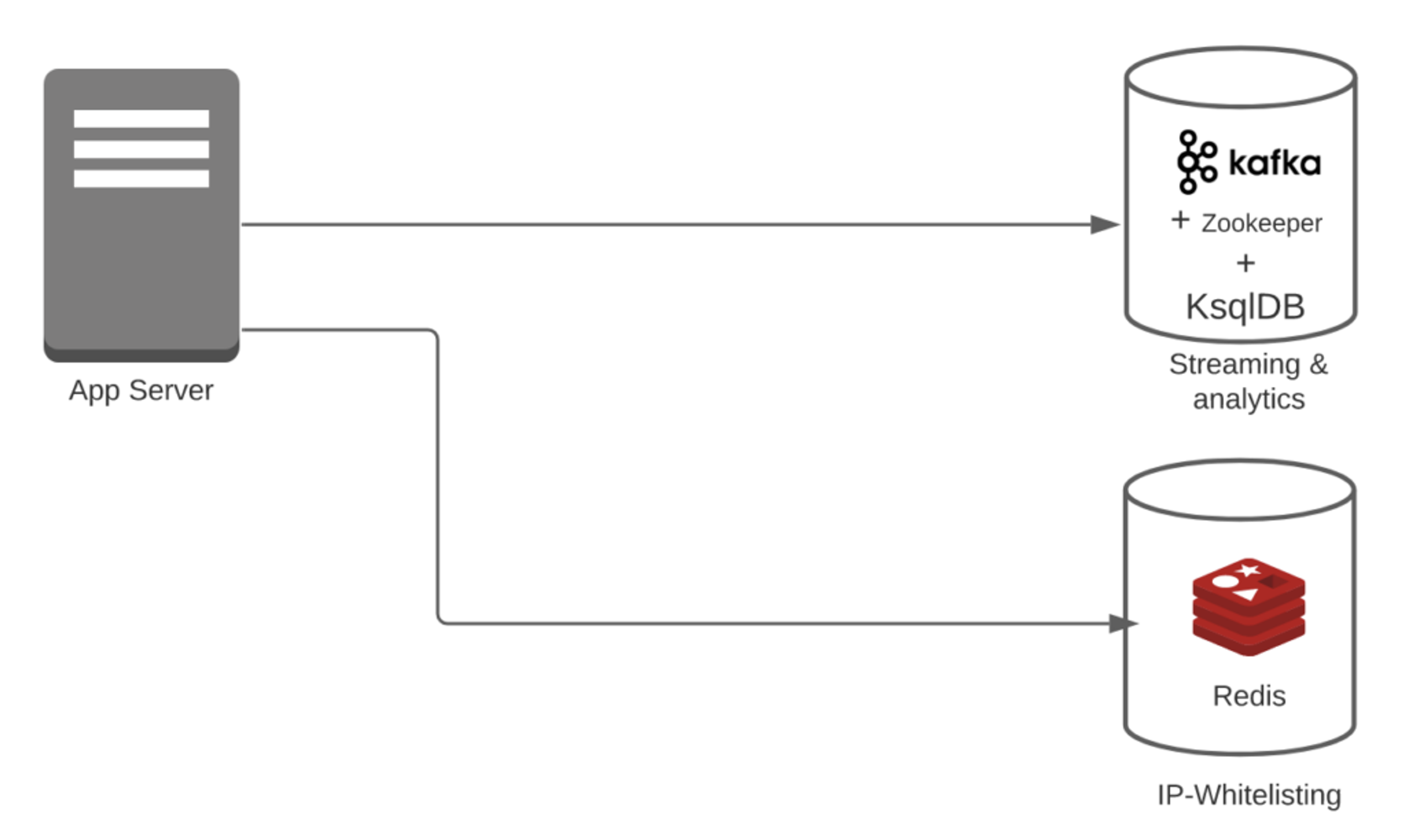
1. Transformational overhead = 0
   1. For IP-whitelisting, you don’t need any transformation. Also, Kafka and KsqlDB can easily handle streams. 
2. Pipeline overhead = 2
   1. You have Redis + (Kafka + KsqlDB). Note: In this case, we are considering Kafka + KsqlDB part of the same system.
3. Number of features = 2

Case 4: Say you are using Redis + Redis Streams + RedisTimeSeries. 

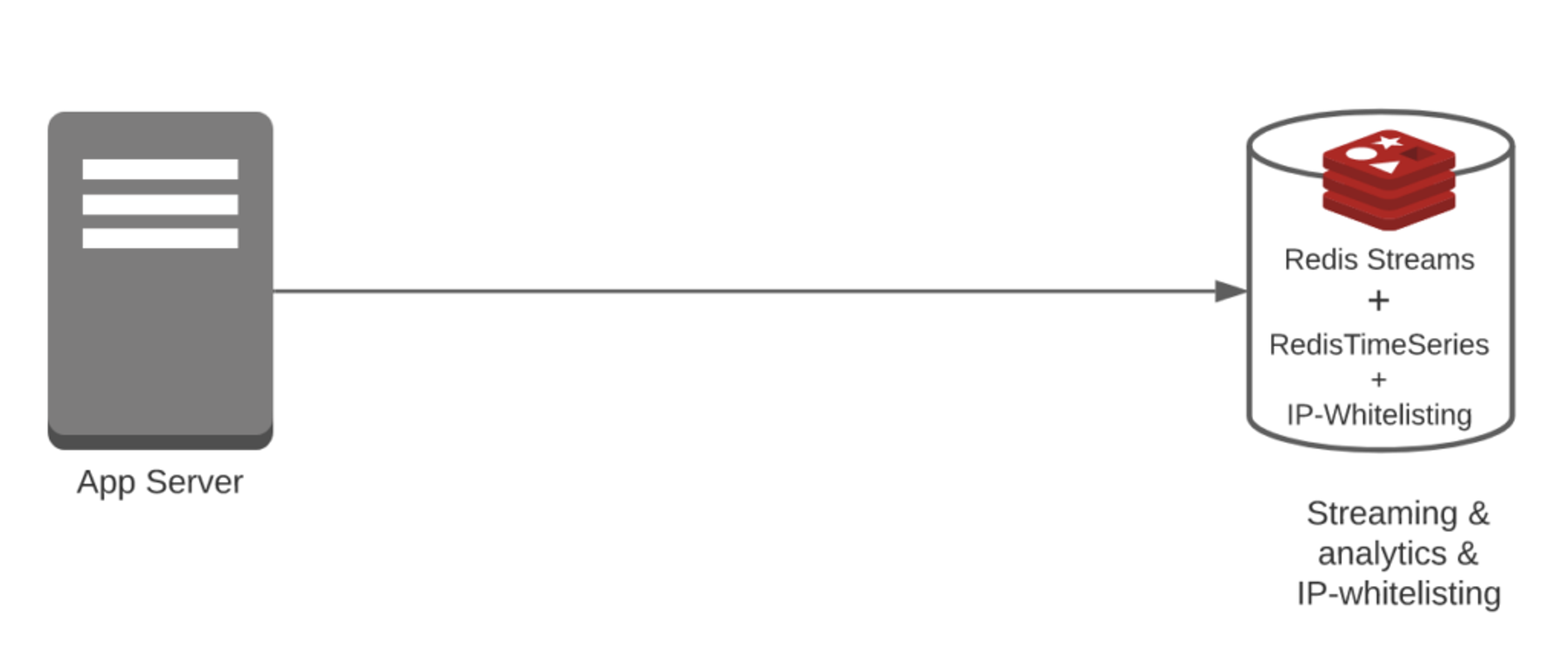
1. Transformational overhead = 0
   1. For IP-whitelisting, you don’t need any transformation. Also, Redis Streams and RedisTimeseries can easily handle streams and alerts.
2. Pipeline overhead = 1
   1. You have Redis +  Redis Streams + Redis TimeSeries. Note: In this case, all three are part of the same system.
3. Number of features = 2

Conclusion after Phase 2: 

When we added an additional feature, 

• Case 1 was at 2 in Phase-1 and went down to 1.5. 
• Case 2 was at 3 in Phase-1 and went down to 2
• Case 3 was at 1 in Phase-1 and remained at 1
• Case 4 was at 1 in Phase-1 and went down to 0.5 (Best)

So in our example, Case 4, which had one of the lowest IMS scores of 1, actually got better as we added the new feature and it ended up at 0.5.  

Please note: If you add more or different features, Case 4 may not remain the simplest. But that’s the idea of the IMS score. Simply list all the features, compare different architectures, and see which one is the best for your use case.

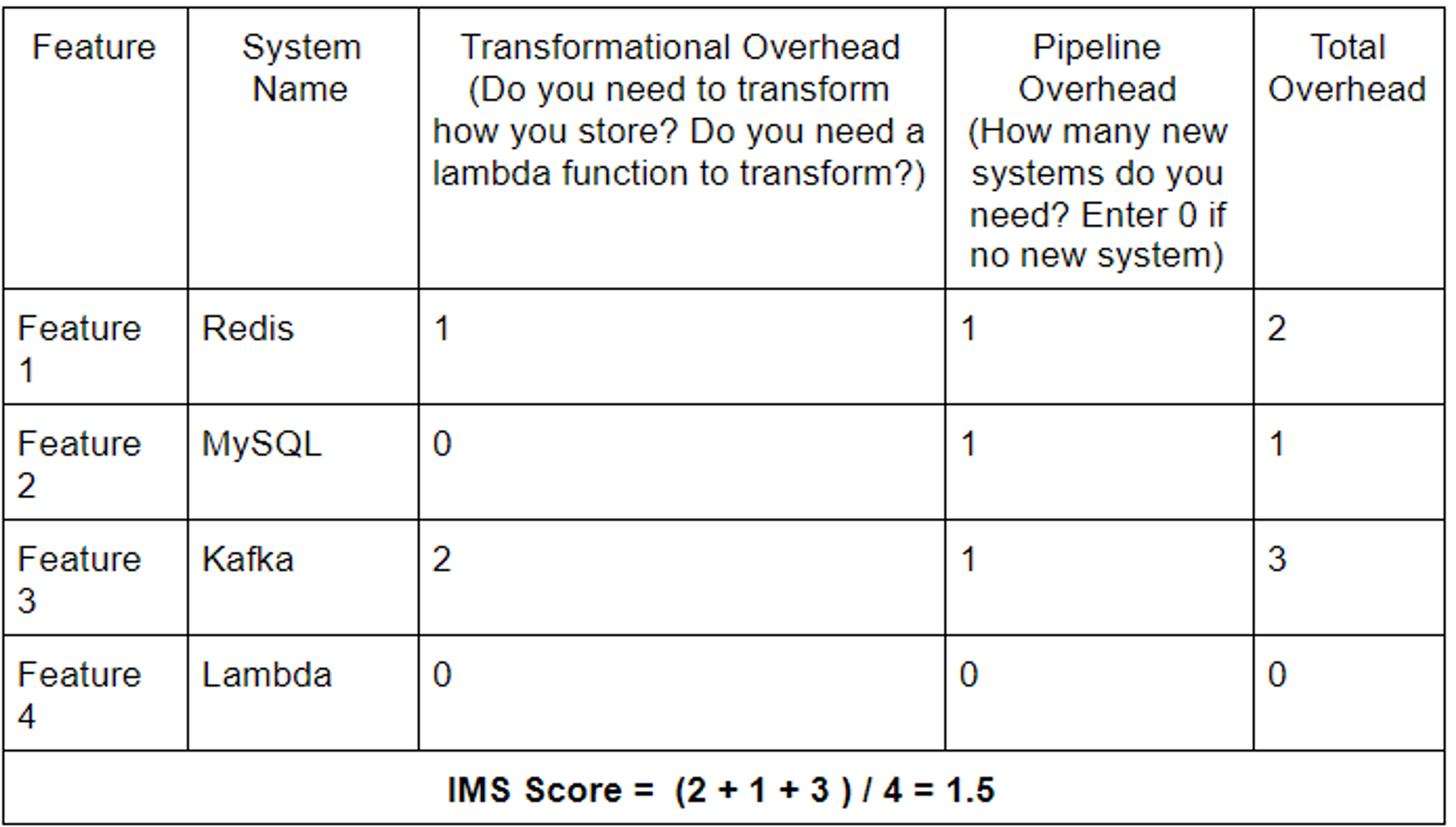
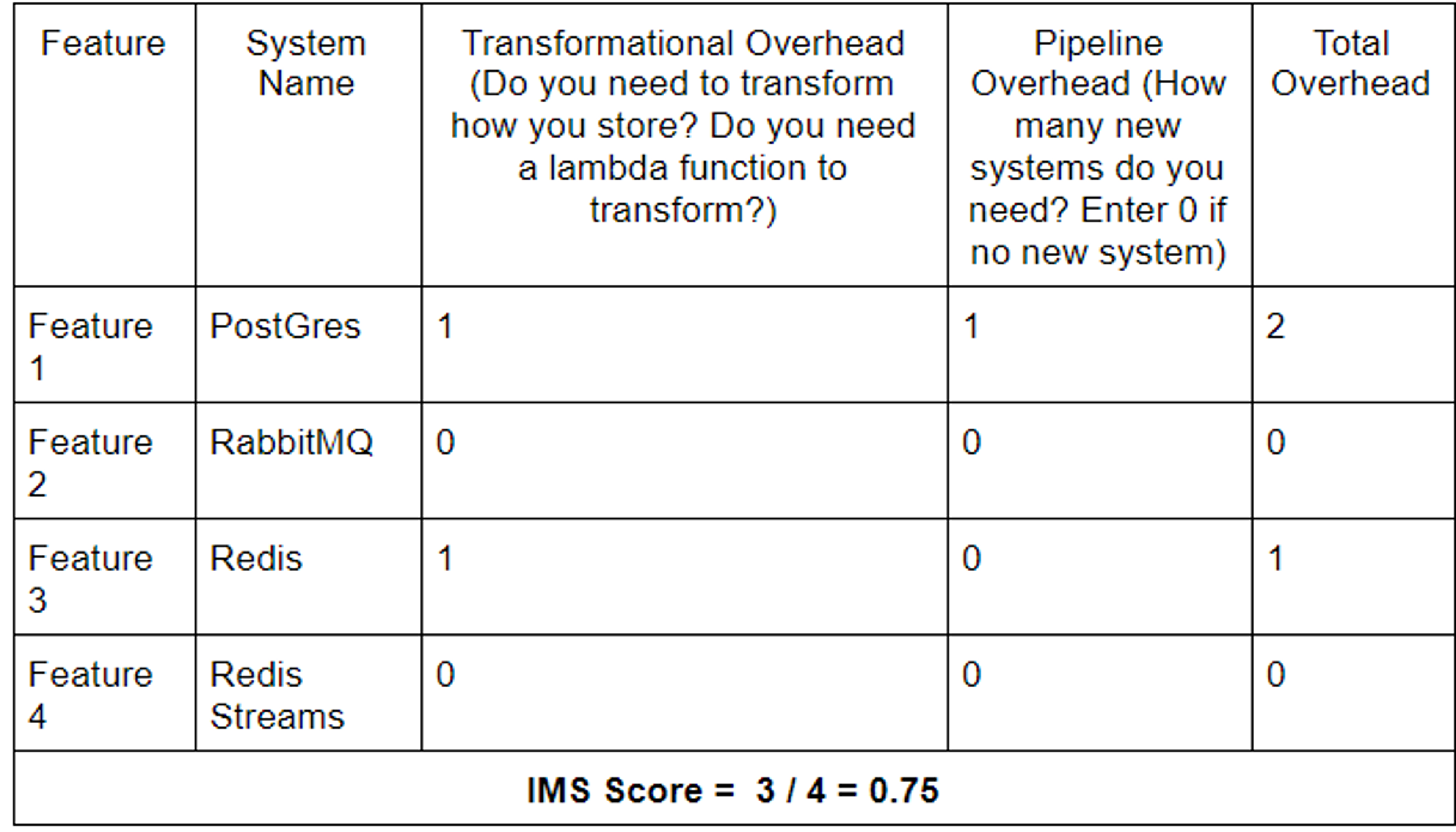
To make it even simpler to use, we are providing you a calculator that you can implement in a simple spreadsheet to calculate the IMS score.

IMS Calculator

Here is how you use it:

1. For each data layer or data pipeline, simply list out:
   1. Features you currently have. 
   2. Features that are in the roadmap. This is important, because you want to make sure that your data layer can continue to support upcoming features without any additional overheads.
2. Then map the Transformational overhead and the Pipeline overhead for each feature.
3. And finally, divide the sum of all the overheads by the number of features.
4. Repeat steps 2 and 3 for pipelines with different systems to compare and contrast them.

Data Pipeline 1

Data Pipeline 2

Summary

It is very easy to get carried away and build a complex data layer without thinking about the consequences. The IMS score was created to help you be conscious of your decision. 

You can use the IMS score to easily compare and contrast multiple systems for your use case and see which one is really the best for your set of features. You can also validate if your system can hold up to feature expansions and continue to remain as simple as possible. 

Always remember:

“Simplicity is the ultimate sophistication”  — Leonardo da Vinci

“Most information is irrelevant and most effort is wasted, but only the expert knows what to ignore” — James Clear, Atomic Habits