Collaborative filtering: How to build a recommender system

When users sit down to watch a movie on Netflix, they face a problem untold numbers of Netflix users have faced before: What to watch next? Luckily, the fact that so many users face this problem yet watch another one provides a solution: Collaborative filtering.

With collaborative filtering, recommender systems—often powered by machine learning, deep learning, and artificial intelligence—can use interactions from different users, like ratings, to inform recommendations for other users.

In an ideal world, this looks like magic. A user opens up Netflix, and without realizing it, a similar user selected a movie previously, and that decision helps the recommendation algorithm to infer what the original user might like.

But under the hood, collaborative filtering is anything but magic.

What is collaborative filtering?

Collaborative filtering was one of the first approaches used to build recommender systems. Collaborative filtering, at its core, relies on user interactions, such as user ratings, user likes, user dislikes, and purchases, to make recommendations.

Collaborative filtering gets its name from the way this approach allows users to “collaborate” with each other via implicit feedback. One user doesn’t need to know the other to help them by rating a movie highly so that the system can recommend it to the next user.

It’s tempting to think of recommender systems—the behind-the-scenes tools that seem to magically know what users want to buy, watch, or see next—as entirely modern systems. But recommender systems emerged long before AI, machine learning, and algorithm competitions.

The first recommender system emerged soon after the initial invention of the World Wide Web. While other, more visible systems and concepts have swept over the industry and then been swept away by newer systems and concepts, recommender systems have remained. Over the years, the sophistication of the technologies involved has evolved dramatically, but the challenge of recommending new things to engaged users has always been a challenge.

Collaborative filtering is split into two approaches: User-user and item-item.

In user-user (or user-based) approaches, the recommender system predicts a user’s preferences by finding other users with similar interests or tastes and then recommending similar items on that basis. In item-item (or item-based) approaches, the recommender system uses matrix factorization to suggest new items to users based on how similar those new items are to the previous items they’ve already demonstrated interest in.

Collaborative filtering vs. content-based filtering

Collaborative filtering is not the only approach to building recommender systems.

Content-based filtering, unlike collaborative filtering, which focuses on users, focuses on the content of the items being recommended. In content-based filtering, machine learning algorithms suggest similar items to users based on the content of these items. These recommender systems build user profiles over time and match new items to those profiles with the hopes that users like them, too.

Collaborative filtering, in contrast, focuses on users instead of items and uses explicit feedback from users rather than implicit metadata regarding the items.

Advantages and disadvantages of collaborative filtering

There are advantages and disadvantages to each approach, but many recommender systems use both and treat them as complementary (such as when building hybrid recommender systems). Whether you emphasize one over the other or combine them both, knowing the tradeoffs of each is essential to building a modern recommender system.

Advantages of collaborative filtering

Collaborative filtering has numerous advantages that have made it a long-standing part of recommender systems over the years:

Diverse recommendations: Content-based filtering techniques can sometimes put users into what’s known as “filter bubbles,” where recommendation diversity is limited. Collaborative filtering, assuming there are enough users in the network, can help create better recommendation diversity because one user might enjoy a broad range of items that a similar user might be wholly unfamiliar with.
Network effects: Content-based filtering techniques, even with perfectly detailed metadata, are limited by the number of items. Collaborative filtering techniques, in contrast, benefit from network effects—as new users join the network, recommendations get better and better.
Little data dependency: Content-based filtering techniques tend to need significant amounts of metadata to work well, whereas collaborative filtering techniques—because they focus on users—can work despite data sparsity.

Despite these compelling advantages, collaborative filtering isn’t without its disadvantages.

Disadvantages

Collaborative filtering has some major tradeoffs that companies investing in it need to consider, especially younger companies with newer networks.

Cold-start problem: Collaborative filtering often struggles to surmount the cold-start problem when there are too few users to support compelling recommendations. Content-based filtering, in contrast, needs few users because it focuses on the content of the recommended items.
Computational intensity: Since collaborative filtering relies on a vast number of users, it can become computationally intense as the number of users and items grows.
Bias and trends: Collaborative filtering focuses on what other users want and prefer, which can sometimes lead to weak recommendations based on waves of user behavior or popularity trends. A hit song in a streaming platform could, for example, convince the system that everyone needs to hear the song even if it’s not a fit for many users.

The advantages and disadvantages described above carry more weight once implemented, which you can see via use cases and examples.

Use cases for collaborative filtering

The use cases for collaborative filtering are broad and diverse. Like content-based filtering, collaborative filtering (and all other recommender system techniques) face the same persistent problem: Online, there are always too many options, and too many options lead users to analysis paralysis.

Anywhere that dynamic is possible, you’re likely to find recommender systems and, often, collaborative filtering in particular.

Ecommerce platforms: Ecommerce stores are not bound by physical shelves and can offer a near-infinite number of options. As a result, ecommerce platforms like Amazon often recommend items to users based on similar users’ shopping habits. Shopify, as another example, wrote in a blog post that “CF allows us to leverage past user-item interactions to predict the relevance of each item to a given user. This is based on the assumption that users with similar past behavior will show similar preferences for items in the future.”
Streaming services: Streaming services, including Netflix, Spotify, and others, often use collaborative filtering to suggest new content to watch or listen to based on the behavior patterns of similar users. The most famous collaborative filtering system ever, for example, is Netflix’s because the company launched a $1,000,000 reward for anyone who could beat its in-house collaborative filtering algorithm back in 2009.
Social networks: Social networks, by definition, rely on amassing many users and leveraging network effects, making them a natural fit for collaborative filtering. In a blog post on the topic, Facebook revealed that, in 2015, the “average data set for CF has 100 billion ratings, more than a billion users, and millions of items.”

Collaborative filtering is an old idea (at least in technology terms), and the industry’s methods of building with it and iterating on it have changed over the years. Learning to build a collaborative filtering system yourself is a great first step to building, or at least better understanding, how modern recommender systems work.

How to build a collaborative filtering system with Redis

With Redis, you use real-time, low-latency capabilities to build scalable, AI-powered recommendation systems. In environments where real-time data processing is necessary to make the best recommendations, Redis’ sub-millisecond response times and vector database capabilities can help you deliver seamless user experiences.

Here, we’ll walk through how to build a movie recommendation system supported by collaborative filtering using RedisVL and the IMDB movie dataset.

You can run it yourself or clone the repo here.

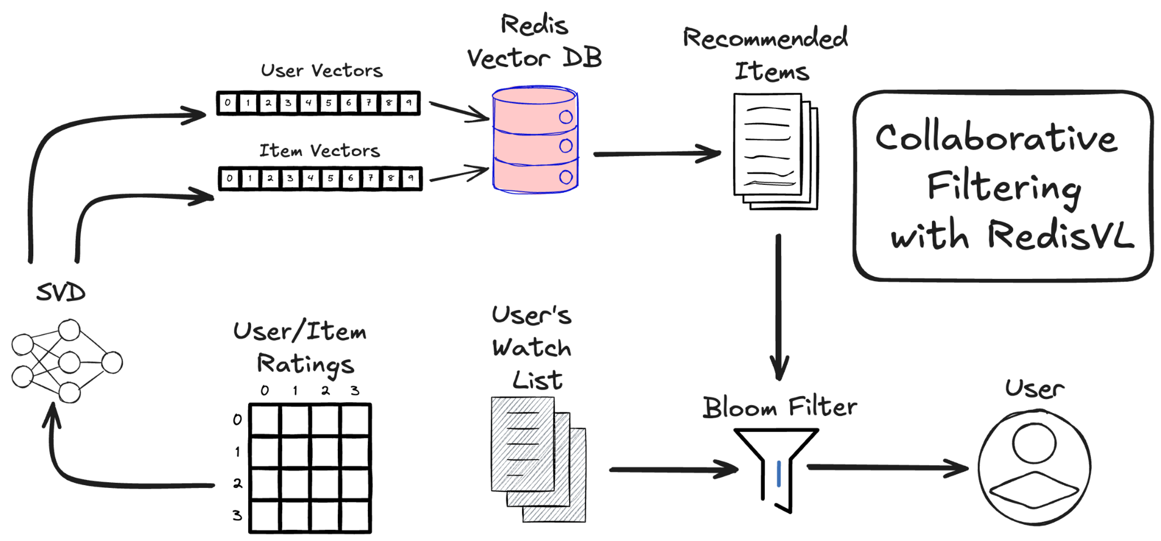
The algorithm we’ll be using is the Singular Value Decomposition, or SVD, algorithm. It works by looking at the average ratings users have given to movies they have already watched. Below is a sample of what that data might look like.

User ID	Movie ID	Rating (0 to 5)
1	31	2.5
1	1029	3.0
1	1061	3.0
1	1129	2.0
1	1172	4.0
2	10	4.0
2	17	5.0
3	60	3.0
3	110	4.0
3	247	3.5
3	267	3.0
3	296	4.5
3	318	5.0
…	…	…

Unlike content filtering, which is based on the features of the recommended items, collaborative filtering looks at the user’s ratings and only the user’s ratings.

Singular value decomposition

It’s worth going into more detail about why we chose this algorithm and what it is computing in the methods we’re calling.

First, let’s think about what data it’s receiving—our ratings data. This only contains the user IDs, movie IDs, and the user’s ratings of the movies they watched on a scale of 0 to 5. We can put this data into a matrix with rows being users and columns being movies.

RATINGS	Movie 1	Movie 2	Movie 3	Movie 4	Movie 5	Movie 6	…
User 1	4	1		4		5
User 2		5	5	2	1
User 3					1
User 4	4	1		4		?
User 5		4	5	2
…

Our empty cells are missing ratings—not zeros—so user 1 has never rated movie 3. They may like it or hate it.

Unlike content-based filtering, here, we only consider the ratings that users assign. We don’t know the plot, genre, or release year of any of these films. However, we can still build a recommender by assuming that users have tastes similar to each other.

As an intuitive example, we can see that user 1 and user 4 have very similar ratings on several movies, so we can assume that user 4 will rate movie 6 highly, just as user 1 did.

Since we only have this matrix to work with, what we want to do is decompose it into two constituent matrices.

Let’s call our ratings matrix [R]. We want to find two other matrices, a user matrix [U] and a movies matrix [M], that fit the equation:

[U] * [M] = [R]

[U] will look like:

User 1 feat 1	User 1 feat 2	User 1 feat 3	User 1 feat 4	…	User 1 feat k
User 2 feat 1	User 2 feat 2	User 2 feat 3	User 2 feat 4	…	User 2 feat k
User 3 feat 1	User 3 feat 2	User 3 feat 3	User 3 feat 4	…	User 3 feat k
…	…	…	…	…	…
User N feat 1	User N feat 2	User N feat 3	User N feat 4	…	User N feat k

[M] will look like:

Movie 1 feat 1	Movie 2 feat 1	Movie 3 feat 1	Movie 4 feat 1	…	Movie M feat 1
Movie 1 feat 2	Movie 2 feat 2	Movie 3 feat 2	Movie 4 feat 2		Movie M feat 2
Movie 1 feat 3	Movie 2 feat 3	Movie 3 feat 3	Movie 4 feat 3		Movie M feat 3
Movie 1 feat 4	Movie 2 feat 4	Movie 3 feat 4	Movie 4 feat 4		Movie M feat 4
…	…	…			…
movie 1 feat k	Movie 2 feat k	Movie 3 feat k	Movie 4 feat 4		Movie M feat k

These features are the latent features (or latent factors) and are the values we’re trying to find when we call the svd.fit(train_set) method. The algorithm that computes these features from our ratings matrix is the SVD algorithm.

Our data sets the number of users and movies. The size of the latent feature vectors k is a parameter we choose. We’ll keep it at the default 100 for this notebook.

A look at the code

Grab the ratings file and load it up with Pandas.

import os
import requests
import pandas as pd
from surprise import SVD
from surprise import Dataset, Reader
 
# we'll be downloading a few files for this example so here's a helper function
def fetch_dataframe(file_name):
    try:
        df = pd.read_csv('datasets/collaborative_filtering/' + file_name)
    except:
        url = 'https://redis-ai-resources.s3.us-east-2.amazonaws.com/recommenders/datasets/collaborative-filtering/'
        r = requests.get(url + file_name)
        if not os.path.exists('datasets/collaborative_filtering'):
            os.makedirs('datasets/collaborative_filtering')
        with open('datasets/collaborative_filtering/' + file_name, 'wb') as f:
            f.write(r.content)
        df = pd.read_csv('datasets/collaborative_filtering/' + file_name)
    return df
 
# for a larger dataset use 'ratings.csv'
ratings_df = fetch_dataframe('ratings_small.csv')
 
# only keep the columns we need: userId, movieId, rating
ratings_df = ratings_df[['userId', 'movieId', 'rating']]
 
reader = Reader(rating_scale=(0.0, 5.0))
ratings_data = Dataset.load_from_df(ratings_df, reader)

A lot is going to happen in the code cell below. We split our full data into train and test sets. We define the collaborative filtering algorithm to use, which in this case is the Singular Value Decomposition (SVD) algorithm. Lastly, we fit our model to our data.

# split the data into training and testing sets (80% train, 20% test)
train_set, test_set = train_test_split(ratings_data, test_size=0.2)
 
# use SVD (Singular Value Decomposition) for collaborative filtering
svd = SVD(n_factors=100, biased=False)  # we'll set biased to False so that predictions are of the form "rating_prediction = user_vector * item_vector"
 
# train the algorithm on the train_set
svd.fit(train_set)

Extract the user and movie vectors

Now that the SVD algorithm has computed our [U] and [M] matrices, which are both just lists of vectors, we can load them into our Redis instance. The Surprise SVD model stores user and movie vectors in two attributes:

svd.pu: user features matrix—a matrix where each row corresponds to the latent features of a user).

svd.qi: item features matrix—a matrix where each row corresponds to the latent features of an item/movie).

It’s worth noting that the matrix svd.qi is the transposition of the matrix [M] we defined above. This way, each row corresponds to one movie.

user_vectors = svd.pu  # user latent features (matrix)
movie_vectors = svd.qi  # movie latent features (matrix)
 
print(f'we have {user_vectors.shape[0]} users with feature vectors of size {user_vectors.shape[1]}')
print(f'we have {movie_vectors.shape[0]} movies with feature vectors of size {movie_vectors.shape[1]}')

we have 671 users with feature vectors of size 100
we have 8397 movies with feature vectors of size 100

Predict user ratings in one step

The great thing about collaborative filtering is that using our user and movie vectors, we can predict the rating any user will give to any movie in our dataset. And unlike content filtering, there is no assumption that all the movies a user will be recommended are similar to each other. A user can get recommendations for dark horror films and light-hearted animations.

Looking back at our SVD algorithm, the equation is:

[User_features] * [Movie_features].transpose = [Ratings]

To predict how a user will rate a movie they haven’t seen yet, we just need to take the dot product of that user’s feature vector and a movie’s feature vector.

# surprise casts userId and movieId to inner ids, so we have to use their mapping to know which rows to use
inner_uid = train_set.to_inner_uid(347) # userId
inner_iid = train_set.to_inner_iid(5515) # movieId
 
# predict one user's rating of one film
predicted_rating = np.dot(user_vectors[inner_uid], movie_vectors[inner_iid])
print(f'the predicted rating of user {347} on movie {5515} is {predicted_rating}')

the predicted rating of user 347 on movie 5515 is 1.1069607933289707

Add movie metadata to our recommendations

While our collaborative filtering algorithm was trained solely on users’ ratings of movies and doesn’t require any data about the movies themselves, such as the title, genre, or release year, we’ll want that information stored as metadata.

We can grab this data from our `movies_metadata.csv` file, clean it, and join it to our user ratings via the `movieId` column.

# fetch and clean the movies data
import datetime
movies_df = fetch_dataframe('movies_metadata.csv')
 
movies_df.drop(columns=['homepage', 'production_countries', 'production_companies', 'spoken_languages', 'video', 'original_title', 'video', 'poster_path', 'belongs_to_collection'], inplace=True)
 
# drop rows that have missing values
movies_df.dropna(subset=['imdb_id'], inplace=True)
 
movies_df['original_language'] = movies_df['original_language'].fillna('unknown')
movies_df['overview'] = movies_df['overview'].fillna('')
movies_df['popularity'] = movies_df['popularity'].fillna(0)
movies_df['release_date'] = movies_df['release_date'].fillna('1900-01-01').apply(lambda x: datetime.datetime.strptime(x, "%Y-%m-%d").timestamp())
movies_df['revenue'] = movies_df['revenue'].fillna(0)
movies_df['runtime'] = movies_df['runtime'].fillna(0)
movies_df['status'] = movies_df['status'].fillna('unknown')
movies_df['tagline'] = movies_df['tagline'].fillna('')
movies_df['title'] = movies_df['title'].fillna('')
movies_df['vote_average'] = movies_df['vote_average'].fillna(0)
movies_df['vote_count'] = movies_df['vote_count'].fillna(0)
movies_df['genres'] = movies_df['genres'].apply(lambda x: [g['name'] for g in eval(x)] if x != '' else []) # convert to a list of genre names
movies_df['imdb_id'] = movies_df['imdb_id'].apply(lambda x: x[2:] if str(x).startswith('tt') else x).astype(int) # remove leading 'tt' from imdb_id

We’ll have to map these movies to their ratings, which we’ll do so with the `links_small.csv` file that matches `movieId`, `imdbId`, and `tmdbId`.

links_df = fetch_dataframe('links_small.csv') # for a larger example use 'links.csv' instead
 
movies_df = movies_df.merge(links_df, left_on='imdb_id', right_on='imdbId', how='inner')

We’ll want to move our SVD user vectors and movie vectors and their corresponding userId and movieId into two dataframes for later processing.

# place movie vectors and their movieIds in a dataframe
movie_vectors_and_ids = {train_set.to_raw_iid(inner_id): movie_vectors[inner_id].tolist() for inner_id in train_set.all_items()}
movie_vector_df = pd.Series(movie_vectors_and_ids).to_frame('movie_vector')
 
# merge the movie vector series with the movies dataframe using movieId and id fields
movies_df = movies_df.merge(movie_vector_df, left_on='movieId', right_index=True, how='inner')
movies_df['movieId'] = movies_df['movieId'].apply(lambda x: str(x)) # need to cast to a string as this is a tag field in our search schema
movies_df.head()
his is a tag field in our search schema
movies_df.head()

RedisVL handles the scale

Especially for large datasets like the 45,000 movie catalog, like the one we’re dealing with here, you’ll want Redis to do the heavy lifting of vector search. All that you need is to define the search index and load the data we’ve cleaned and merged with our vectors.

from redis import Redis
from redisvl.schema import IndexSchema
from redisvl.index import SearchIndex
 
client = Redis.from_url(<REDIS_URL>) # ex: "redis://localhost:6379"
 
schema = {
  "index": {
    "name": "movies",
    "prefix": "movie",
    "storage_type": "json"
  },
  "fields": [
    {"name": "title",
     "type": "text",
    },
    {"name": "genres",
     "type": "tag"
    },
    {"name": "revenue",
     "type": "numeric"
    },
    {"name": "release_date",
     "type": "numeric"
    },
    {"name": "popularity",
     "type": "numeric"
    },
    {"name": "vote_average",
     "type": "numeric"
    },
    {"name": "movie_vector",
     "type": "vector",
     "attrs": {
            "dims": 100,
            "distance_metric": "ip",
            "algorithm": "flat",
            "datatype": "float32"
        }
    }
  ]
}
 
movie_schema = IndexSchema.from_dict(schema)
 
movie_index = SearchIndex(movie_schema, redis_client=client)
movie_index.create(overwrite=True, drop=True)
 
movie_keys = movie_index.load(movies_df.to_dict(orient='records'))

For a complete solution, we’ll store the user vectors and their watched list in Redis, too. We won’t be searching over these user vectors, so there is no need to define an index for them. A direct JSON look up will do.

from redis.commands.json.path import Path
 
# collect the user vectors and their userIds
user_vectors_and_ids = {train_set.to_raw_uid(inner_id): user_vectors[inner_id].tolist() for inner_id in train_set.all_users()}
 
# use a Redis pipeline to store user data and verify it in a single transaction
with client.pipeline() as pipe:
 for user_id, user_vector in user_vectors_and_ids.items():
        user_key = f"user:{user_id}"
        watched_list_ids = ratings_df[ratings_df['userId'] == user_id]['movieId'].tolist()
 
        user_data = {
            "user_vector": user_vector,
            "watched_list_ids": watched_list_ids
        }
        pipe.json().set(user_key, Path.root_path(), user_data)
        pipe.execute()

Unlike in content-based filtering, where we want to compute vector similarity between items and use cosine similarity between items vectors to do so, in collaborative filtering, we instead try to compute the predicted rating a user will give to a movie by taking the inner product of the user and movie vector.

This is why, in our schema definition, we use ‘ip’ (inner product) as our distance metric. It’s also why we’ll use our user vector as the query vector when we do a query. The distance metric ‘ip’ inner product is computing:

vector_distance = 1 – u * v

And it’s returning the minimum, which corresponds to the max of u * v. This is what we want. The predicted rating on a scale of 0 to 5 is then:

predicted_rating= -(vector_distance-1) = –vector_distance +1

Let’s pick a random user and their corresponding user vector to see what this looks like.

from redisvl.query import RangeQuery
 
user_vector = client.json().get(f"user:{352}")["user_vector"]
 
query = RangeQuery(vector=user_vector,
                    vector_field_name='movie_vector',
                    num_results=5,
                    return_score=True,
                    return_fields=['title', 'genres']
                    )
 
results = movie_index.query(query)
 
for r in results:
    # compute our predicted rating on a scale of 0 to 5 from vector distance
    r['predicted_rating'] = - float(r['vector_distance']) + 1.
    print(f"vector distance: {float(r['vector_distance']):.08f},\t predicted rating: {r['predicted_rating']:.08f},\t title: {r['title']}, ")
 
 
 
vector distance: -3.63527393,    predicted rating: 4.63527393,   title: Fight Club, 
vector distance: -3.60445881,    predicted rating: 4.60445881,   title: All About Eve, 
vector distance: -3.60197020,    predicted rating: 4.60197020,   title: Lock, Stock and Two Smoking Barrels, 
vector distance: -3.59518766,    predicted rating: 4.59518766,   title: Midnight in Paris, 
vector distance: -3.58543396,    predicted rating: 4.58543396,   title: It Happened One Night, 

Add all the bells and whistles

Vector search handles the bulk of our collaborative filtering recommendation system and is a great approach to generating personalized recommendations that are unique to each user.

To up our RecSys game even further, we can use RedisVL Filter logic to get more control over what users are shown. Why have only one feed of recommended movies when you can have several, each with its own theme and personalized to each user?

from redisvl.query.filter import Tag, Num, Text
 
def get_recommendations(user_id, filters=None, num_results=10):
    user_vector = client.json().get(f"user:{user_id}")["user_vector"]
query = RangeQuery(vector=user_vector,
                       vector_field_name='movie_vector',
                       num_results=num_results,
                       filter_expression=filters,
                       return_fields=['title', 'overview', 'genres'])
 
    results = movie_index.query(query)
 
    return [(r['title'], r['overview'], r['genres'], r['vector_distance']) for r in results]
 
Top_picks_for_you = get_recommendations(user_id=42) # general SVD results, no filter
 
block_buster_filter = Num('revenue') > 30_000_000
block_buster_hits = get_recommendations(user_id=42, filters=block_buster_filter)
 
classics_filter = Num('release_date') < datetime.datetime(1990, 1, 1).timestamp()
classics = get_recommendations(user_id=42, filters=classics_filter)
 
popular_filter = (Num('popularity') > 50) & (Num('vote_average') > 7)
Whats_popular = get_recommendations(user_id=42, filters=popular_filter)
 
indie_filter = (Num('revenue') < 1_000_000) & (Num('popularity') > 10)
indie_hits = get_recommendations(user_id=42, filters=indie_filter)
fruity = Text('title') % 'apple|orange|peach|banana|grape|pineapple'
fruity_films = get_recommendations(user_id=42, filters=fruity)
# put all these titles into a single pandas dataframe, where each column is one category
all_recommendations = pd.DataFrame(columns=["top picks", "block busters", "classics", "what's popular", "indie hits", "fruity films"])
all_recommendations["top picks"] = [m[0] for m in Top_picks_for_you]
all_recommendations["block busters"] = [m[0] for m in block_buster_hits]
all_recommendations["classics"] = [m[0] for m in classics]
all_recommendations["what's popular"] = [m[0] for m in Whats_popular]
all_recommendations["indie hits"] = [m[0] for m in indie_hits]
all_recommendations["fruity films"] = [m[0] for m in fruity_films]
all_recommendations.head(10)

Top picks	Blockbusters	Classics	What’s popular	Indie hits	Fruity films
The Shawshank Redemption	Forrest Gump	Cinema Paradiso	The Shawshank Redemption	Castle in the Sky	What’s Eating Gilbert Grape
Forrest Gump	The Silence of the Lambs	The African Queen	Pulp Fiction	My Neighbor Totoro	A Clockwork Orange
Cinema Paradiso	Pulp Fiction	Raiders of the Lost Ark	The Dark Knight	All Quiet on the Western Front	The Grapes of Wrath
Lock, Stock and Two Smoking Barrels	Raiders of the Lost Ark	The Empire Strikes Back	Fight Club	Army of Darkness	Pineapple Express
The African Queen	The Empire Strikes Back	Indiana Jones and the Last Crusade	Whiplash	All About Eve	James and the Giant Peach
The Silence of the Lambs	Indiana Jones and the Last Crusade	Star Wars	Blade Runner	The Professional	Bananas
Pulp Fiction	Schindler’s List	The Manchurian Candidate	The Avengers	Shine	Orange County
Raiders of the Lost Ark	The Lord of the Rings: The Return of the King	The Godfather: Part II	Guardians of the Galaxy	Yojimbo	Herbie Goes Bananas
The Empire Strikes Back	The Lord of the Rings: The Two Towers	Castle in the Sky	Gone Girl	Belle de Jour	The Apple Dumpling Gang

Keep things fresh with Bloom filters

You’ve probably noticed that a few movies get repeated in these lists. That’s not surprising as all our results are personalized, and things like popularity, rating, and revenue are likely highly correlated. And it’s more than likely that at least some of the recommendations we’re expecting to be highly rated by a given user are ones they’ve already watched and rated highly.

We need a way to filter out movies that a user has already seen and movies that we’ve already recommended to them before. We could use a Tag filter on our queries to filter out movies by their ID, but this gets cumbersome quickly.

Luckily, Redis offers an easy answer to keeping recommendations new and interesting: Bloom Filters.

# rewrite the get_recommendations() function to use a bloom filter and apply it before we return results
def get_unique_recommendations(user_id, filters=None, num_results=10):
    user_data = client.json().get(f"user:{user_id}")
    user_vector = user_data["user_vector"]
    watched_movies = user_data["watched_list_ids"]
 
    # filter out movies that the user has already watched
    client.bf().insert('user_watched_list', [f"{user_id}:{movie_id}" for movie_id in watched_movies])
 
    query = RangeQuery(vector=user_vector,
                       vector_field_name='movie_vector',
                       num_results=num_results * 5,  # fetch more results to filter out watched movies
                       filter_expression=filters,
                       return_fields=['title', 'overview', 'genres', 'movieId'],
    )
    results = movie_index.query(query)
 
    matches = client.bf().mexists("user_watched_list", *[f"{user_id}:{r['movieId']}" for r in results])
 
    recommendations = [
        (r['title'], r['overview'], r['genres'], r['vector_distance'], r['movieId'])
        for i, r in enumerate(results) if matches[i] == 0
    ][:num_results]
 
    # add these recommendations to the bloom filter so they don't appear again
    client.bf().insert('user_watched_list', [f"{user_id}:{r[4]}" for r  in recommendations])
    return recommendations

# put all these titles into a single pandas dataframe , where each column is one category
all_recommendations = pd.DataFrame(columns=["top picks", "block busters", "classics", "what's popular", "indie hits"])
all_recommendations["top picks"] = [m[0] for m in top_picks_for_you]
all_recommendations["block busters"] = [m[0] for m in block_buster_hits]
all_recommendations["classics"] = [m[0] for m in classics]
all_recommendations["what's popular"] = [m[0] for m in whats_popular]
all_recommendations["indie hits"] = [m[0] for m in indie_hits]

Top picks	Blockbusters	Classics	What’s popular	Indie hits
Cinema Paradiso	The Manchurian Candidate	Castle in the Sky	Fight Club	All Quiet on the Western Front
Lock, Stock and Two Smoking Barrels	Toy Story	12 Angry Men	Whiplash	Army of Darkness
The African Queen	The Godfather: Part II	My Neighbor Totoro	Blade Runner	All About Eve
The Silence of the Lambs	Back to the Future	It Happened One Night	Gone Girl	The Professional
Eat Drink Man Woman	The Godfather	Stand by Me	Big Hero 6	Shine

Get started with RedisVL

Now you know the basics of collaborative filtering, the advantages and disadvantages of this approach, a range of use cases and examples, and how to build a collaborating filtering system using RedisVL.

With Redis and RedisVL, it only takes a few steps to build a highly scalable, personalized, customizable collaborative filtering recommendation system. Be sure to check out how to build a content-filtering recommendation system if you’re curious about how to do the same for content-based filtering.

Try Redis for free or book a demo to see collaborative filtering and recommender systems in action.