Blog
Benchmarking results for vector databases


At Redis, we’re fast. To show how fast we are, we benchmarked the top providers in the market for vector databases using our new Redis Query Engine, now GA for Redis Software. This feature enhances our engine enabling concurrent access to the index, improving throughput for Redis queries, search, and vector database workloads. This blog post shows our benchmark results, explains the challenges with increasing query throughput, and how we overcame those with our new Redis Query Engine. This blog has three main parts:
- See a detailed comparison of benchmark results across vector databases
- Delves into the architectural design of the new Redis Query Engine
- Read an in-depth look of our testing methodology
Let’s start with what matters most, how fast Redis is.
Redis is the fastest on competitive vector benchmarks.
Next to ingestion and index creation time, we benchmarked two key metrics: throughput and latency (see below the details about the metrics and principles) among 7 vector database players. Throughput indicates a system’s capability to process numerous queries or large datasets in a short amount of time, while latency measures how fast individual similarity searches return results.
To ensure we cover both, we’ve proceeded with two benchmarks, one multi-client benchmark focusing on throughput, and another single-client and under load (multi-client) benchmark focusing on latency. All the results can be filtered in the graphs below and all the details of how we conduct the tests can be explored in the blog. For Redis, prioritizing throughput and latency aligns with our core philosophy of delivering exceptional speed and reliability.
Our tests show that Redis is faster for vector database workloads compared to any other vector database we tested, at recall >= 0.98. Redis has 62% more throughput than the second-ranked database for lower-dimensional datasets (deep-image-96-angular) and has 21% more throughput for high-dimensional datasets (dbpedia-openai-1M-angular).
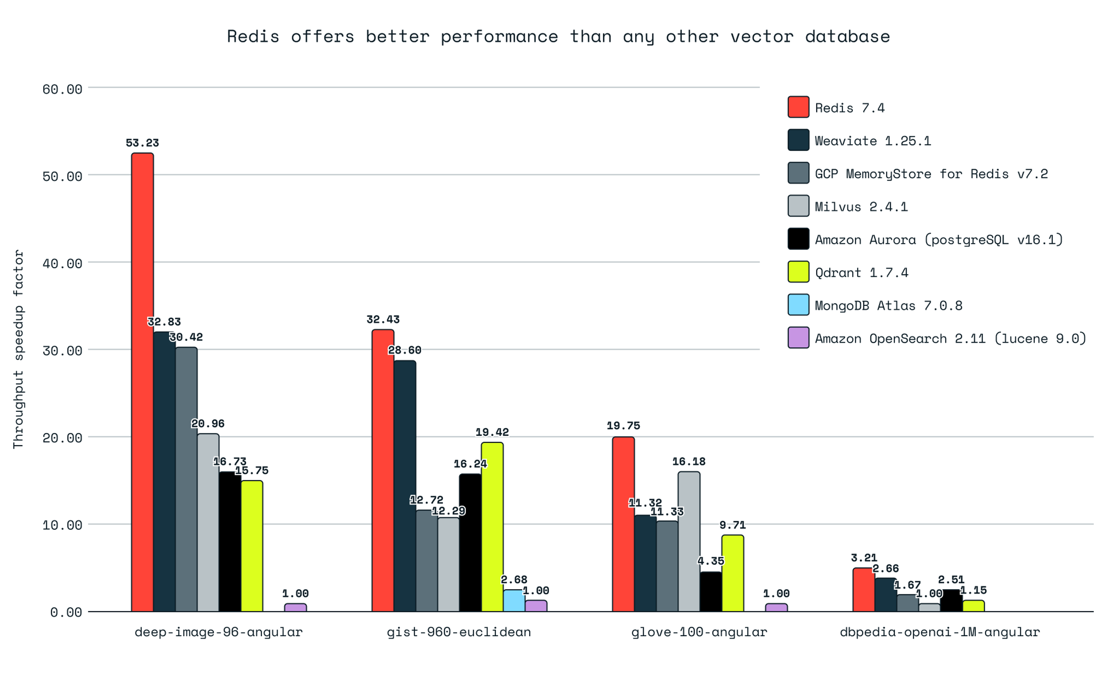
Caveat: MongoDB tests only provided results when using a smaller recall level for the gist-960-euclidean dataset. The results for this dataset considered a median of the results for recall between 0.82 and 0.98. For all other datasets we’re considering recall >=0.98
Our results show we’re faster than any pure vector database providers (Qdrant, Milvus, Weviate).
Redis outperformed other pure vector database providers in querying throughput and latency times.
Querying: Redis achieved up to 3.4 times higher queries per second (QPS) than Qdrant, 3.3 times higher QPS than Milvus, and 1.7 times higher QPS than Weaviate for the same recall levels. On latency, considered here as an average response for the multi-client test, Redis achieved up to 4 times less latency than Qdrant, 4.67 times than Milvus, and 1.71 times faster than Weaviate for the same recall levels. On latency, considered here as an average response under load (multi-client), Redis achieved up to 4 times less latency than Qdrant, 4.67 times than Milvus, and 1.71 times faster than Weaviate.
Ingestion and indexing: Qdrant is the fastest due to its multiple segments index design, but Redis excels in fast querying. Redis showed up to 2.8 times lower indexing time than Milvus and up to 3.2 times lower indexing time than Weaviate.
This section provides a comprehensive comparison between Redis 7.4 and other industry providers that exclusively have vector capabilities such as Milvus 2.4.1, Qdrant 1.7.4, and Weaviate 1.25.1.
In the graph below you can analyze all the results across RPS (request per second), latency (both single-client and multi-client, under load), P95 latency, and index time. All are measured across the different selected datasets.
Pure vector database providers
There were some cases in single client benchmarks in which the performance of Redis and the competitors was at the same level. Weaviate and Milvus showcased operational problems on the cloud setups; findings are fully described in the appendix.
Redis is faster across all data sizes than general-purpose databases (PostgreSQL, MongoDB, OpenSearch).
In the benchmarks for querying performance in general-purpose databases with vector similarity support, Redis significantly outperformed competitors.
Querying: Redis achieved up to 9.5 times higher queries per second (QPS) and up to 9.7 times lower latencies than Amazon Aurora PostgreSQL v16.1 with pgvector 0.5.1 for the same recall. Against MongoDB Atlas v7.0.8 with Atlas Search, Redis demonstrated up to 11 times higher QPS and up to 14.2 times lower latencies. Against Amazon OpenSearch, Redis demonstrated up to 53 times higher QPS and up to 53 times lower latencies.
Ingestion and indexing: Redis showed a substantial advantage over Amazon Aurora PostgreSQL v16.1 with pgvector 0.5.1, with indexing times ranging from 5.5 to 19 times lower.
This section is a comprehensive comparison between Redis 7.4 and Amazon Aurora PostgreSQL v16.1 with pgvector 0.5.1, as well as MongoDB Atlas v7.0.8 with Atlas Search, and Amazon OpenSearch 2.11, offering valuable insights into the performance of vector similarity searches in general-purpose DB cloud environments.
In the graph below you can analyze all the results across RPS (request per second), latency (both single-client and multi-client, under load) and P95 latency, and index time. All are measured across the different selected datasets.
General purpose benchmarks
Apart from the performance advantages showcased above, some general-purpose databases presented vector search limitations related to lack of precision and the possibility of index configuration, fully described in the appendix.
Redis is faster across all data sizes vs. cloud service providers (MemoryDB and MemoryStore).
Compared to other Redis imitators, such as Amazon MemoryDB and Google Cloud MemoryStore for Redis, Redis demonstrates a significant performance advantage. This indicates that Redis and its enterprise implementations are optimized for performance, outpacing other providers that copied Redis.
Querying: Against Amazon MemoryDB, Redis achieved up to 3.9 times higher queries per second (QPS) and up to 4.1 times lower latencies for the same recall. Compared to GCP MemoryStore for Redis v7.2, Redis demonstrated up to 2.5 times higher QPS and up to 4.8 times lower latencies.
Ingestion and indexing: Redis had an advantage over Amazon MemoryDB with indexing times ranging from 1.39 to 3.89 times lower. Against GCP MemoryStore for Redis v7.2, Redis showed an even greater indexing advantage, with times ranging from 4.9 to 10.34 times lower.
In the graph below you can analyze all the results across: RPS (request per second), latency (both single-client and multi-client under load), P95 latency, and index time. All are measured across the different selected datasets.
Cloud service providers
The fastest vector database available leverages the enhanced Redis Query Engine.
To achieve the showcased results, we introduce a new enhancement to enable queries to concurrently access the index. This section elaborates on the enhancements and how our engineering team overcame these challenges.
Single-threading is not optimal for all searches.
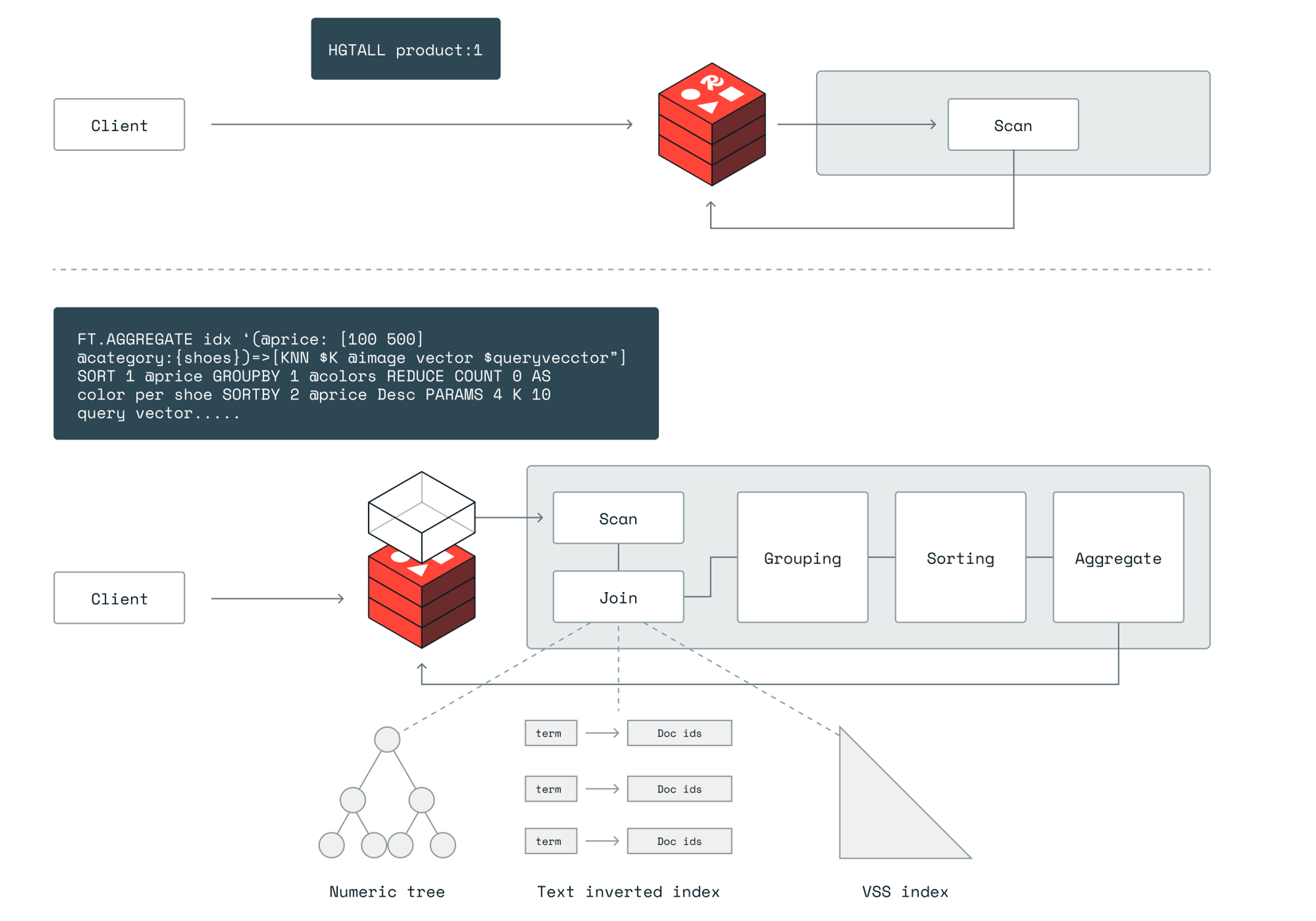
Redis has a proven single-thread architecture and we continually seek improvements to take Redis even further. To do so, we needed to overcome a few constraints of the existing design. First, Redis’ way of scaling, both read and write commands (Redis operations), is based on the assumption that most of the commands are short, usually O(1) time complexity for each command, and are independent of each other. Thus, sharding the data with Redis Cluster into independent Redis shards (or scaling out) causes fanning out multiple requests to multiple shards, so we get immediate load balancing and evenly distribute commands between the shards. That isn’t true for all Redis queries with high expressivity (multiple query terms and conditions) or with any data manipulation (sorting, grouping, transformations). Second, long-running queries on a single thread cause congestion, increase the overall command latency, and drop the Redis server’s overall throughput. Searching in data, leveraging in an inverted index, is one such long-running query, for instance.
Search is not a O(1) time complexity command. Searches usually combine multiple scans of indexes to comply with the several query predicates. Those scans are usually done in logarithmic time complexity O(log(n)) where n is the amount of data points mapped by the index. Having multiple of those, combining their results and aggregating them, is considerably heavier with respect to computing, compared to typical Redis operations for GET, SET, HSET, etc. This is counter to our assumption that commands are simple and have a short runtime.
Horizontal scaling isn’t always sufficient to scale throughput.
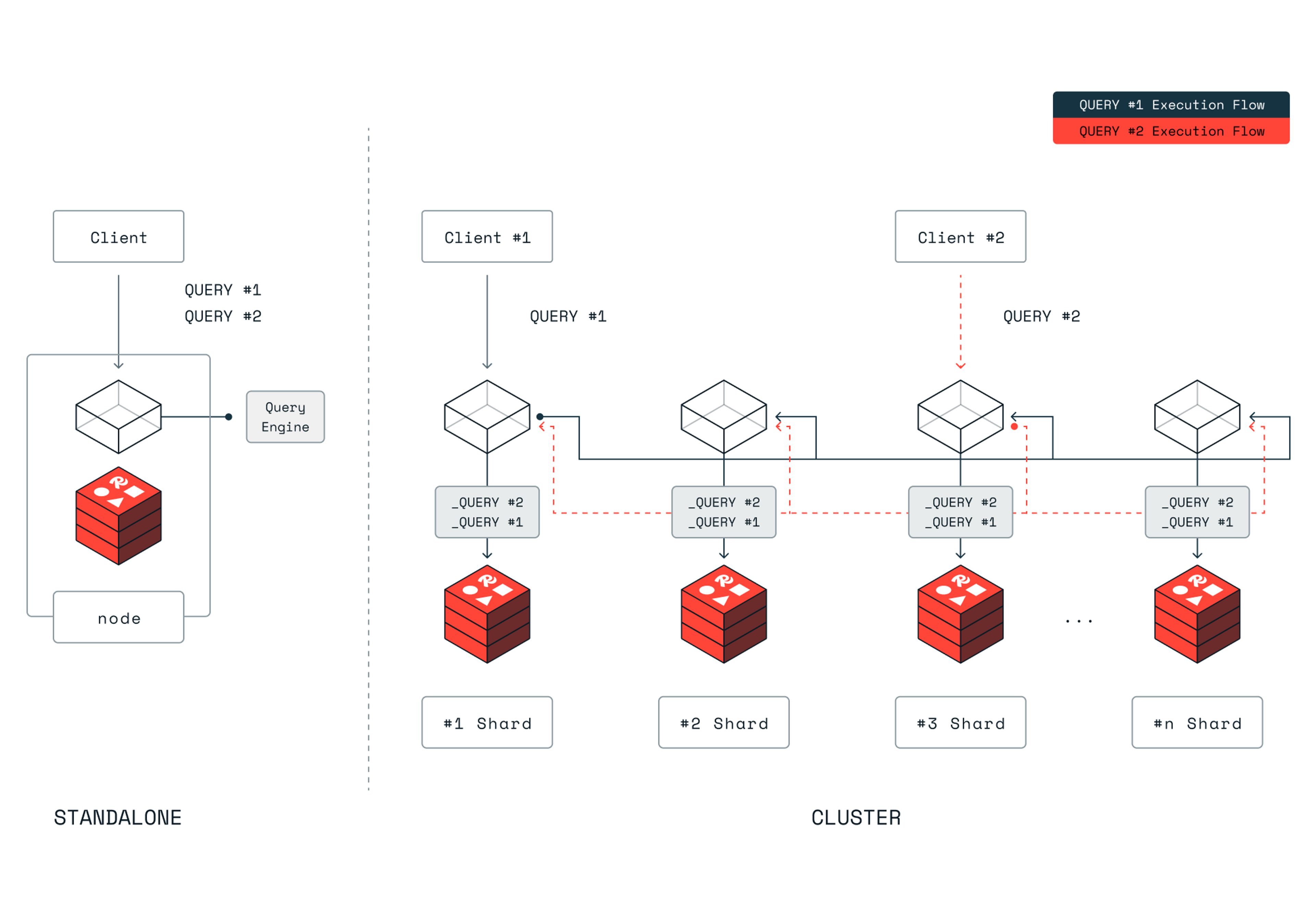
Scaling out with sublinear time complexity doesn’t help reduce the single client latency which is required to increase the throughput in a single-threaded architecture. Even though sharding can distribute data across multiple Redis processes (and nodes), the total query time doesn’t significantly decrease as more shards, and hence more Redis processes, are added. We have two reasons for that.
- The time complexity of index access is often O(log(n)). So for example, splitting the dataset into two shards, and halving the data set into two shards doesn’t reduce the latency in half. Mathematically, O(log(n/2)) is the equivalent of O(log(n)).
- We also have distribution costs, including the overhead of communicating across shards and post-processing sharded results. This scatter and gather cost becomes highly evident when combined with higher concurrency (at high throughput) in a multi-client scenario.
For example, searching for a similar vector today, even with the state-of-art algorithms is compute-heavy since it compares the queried vector to each of the candidate vectors the index provides. This comparison is not a O(1) comparison but is O(d) where d is the vector dimension. In simple terms, each computation is comparing the entire two vectors. This is computer-heavy. When running on the main thread, this holds the Redis’ main thread longer than regular Redis workloads and even other search cases.
Multi-threading improves search speed at scale.
Scaling search efficiently requires combining the distribution of data loads horizontally (going out) and multi-threading vertically, enabling concurrency on accessing the index (going up). The image below illustrates the architecture of a single shard.
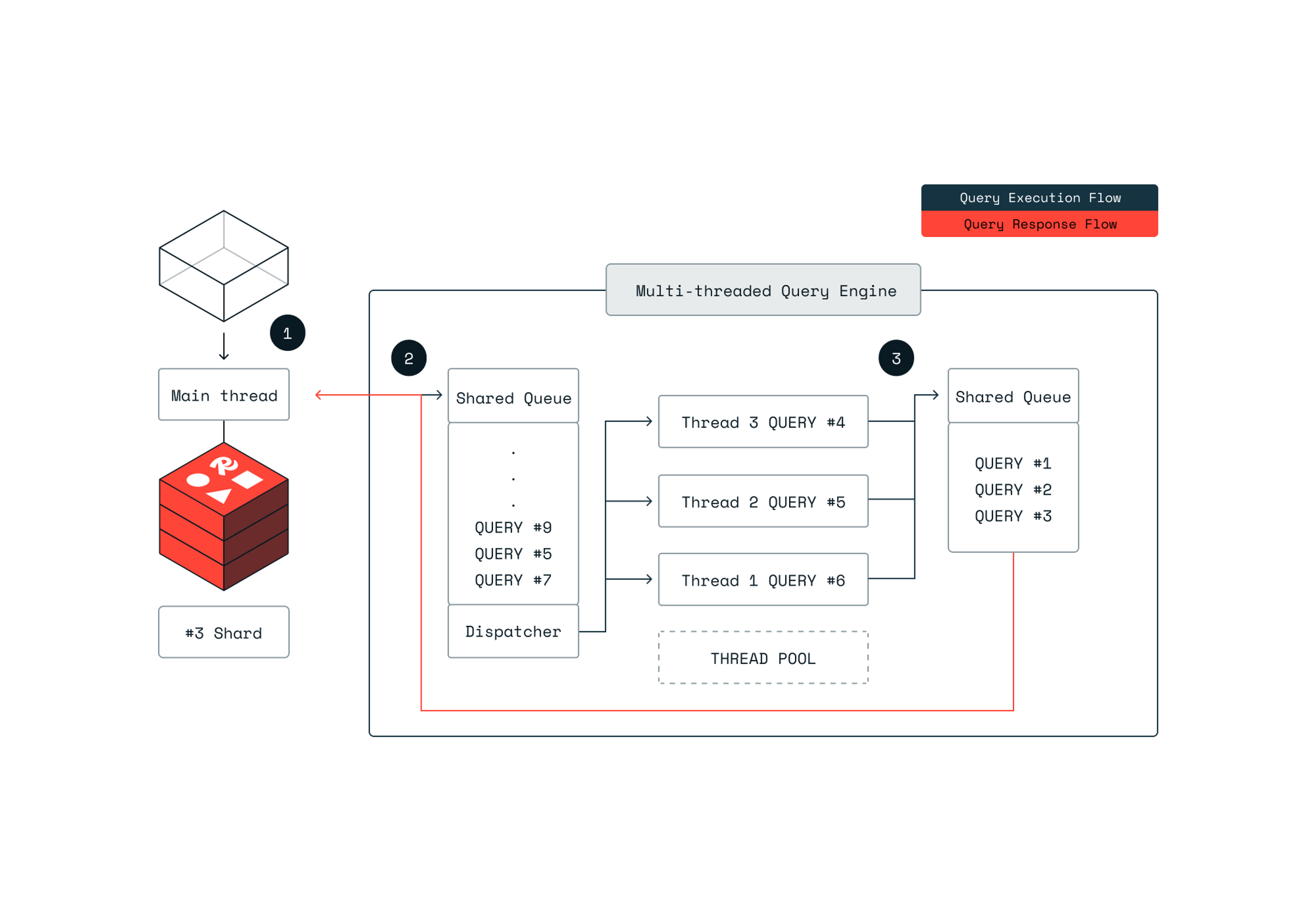
Multiple queries are being executed, each on a separate thread. We incorporated the simple but famous producer-consumer pattern. 1. The query context (planning) is prepared on the main thread and queued on a shared queue. 2. From here, threads consume the queue and execute the query pipeline, concurrently to other threads. This allows us to execute multiple concurrent queries while keeping the main thread alive to handle more incoming requests, such as other Redis commands, or prepare and queue additional queries. 3. Once finished, the query results are sent back to the main thread.
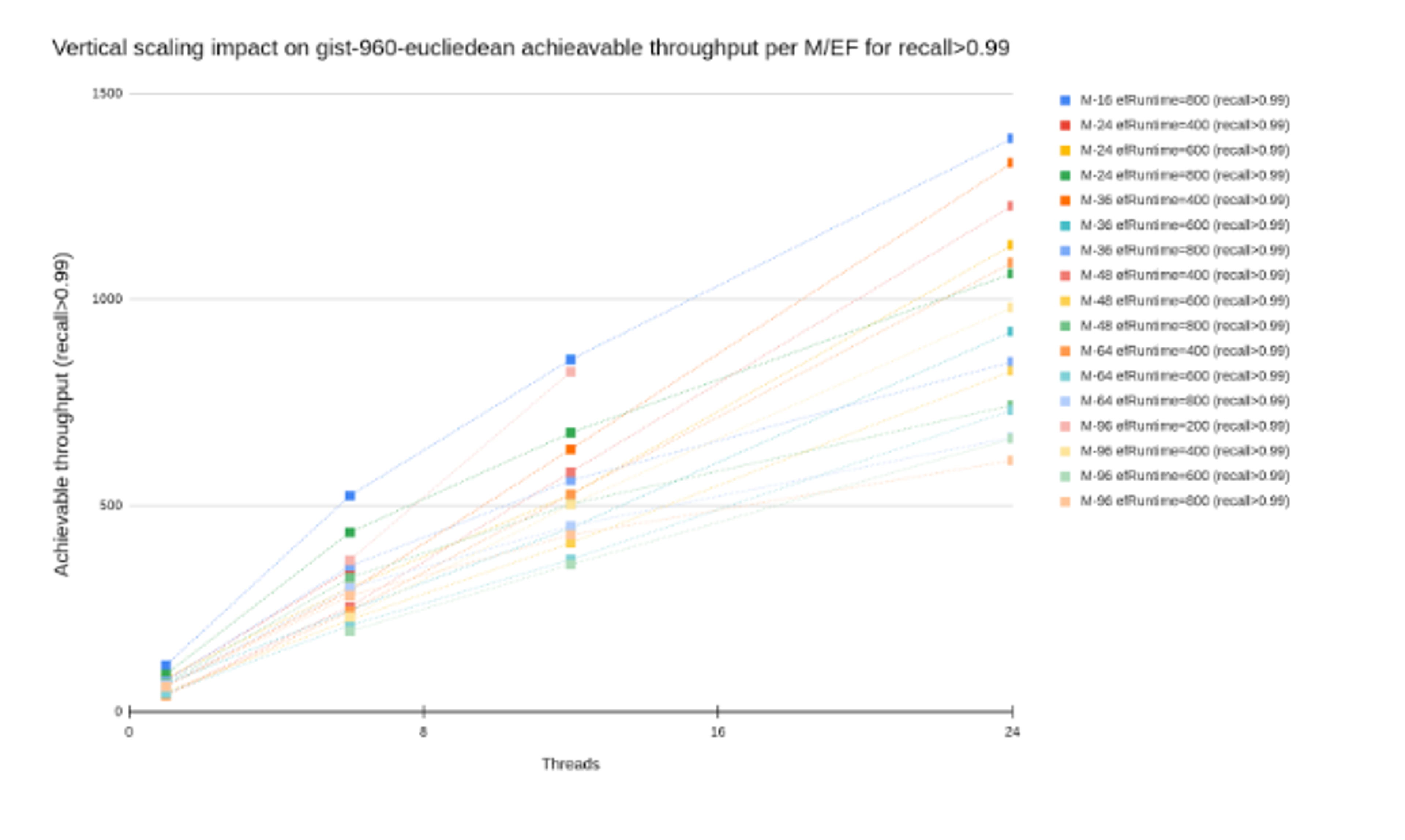
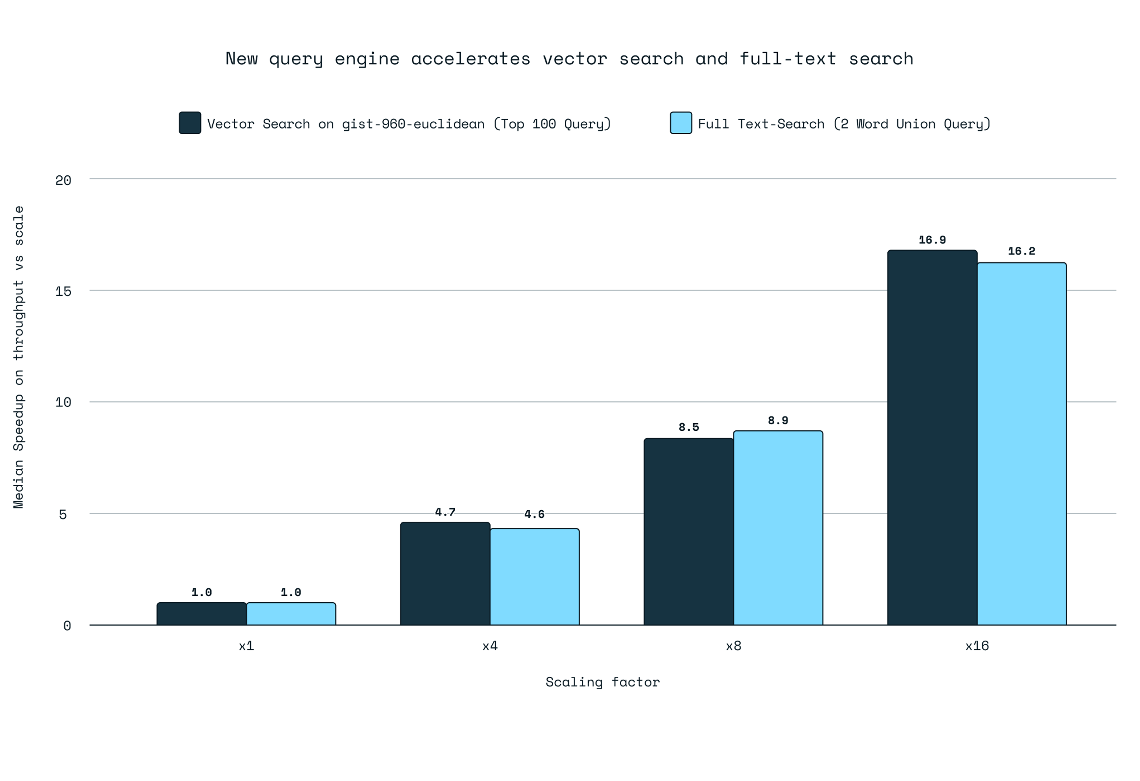
Redis Query Engine scales 16X higher than before.
To benchmark our Redis Query Engine, we’ve tested Redis with both full-text and vector search queries. Specifically for the vector search we’ve picked the gist-960 dataset with 1M vectors, with each vector having 960 dimensions, and compared an old setup with a single shard to a new setup using a thread configuration of 6, 12, and 24, while varying the M (maximum number of connections per node) and EF (the size of the dynamic candidate list during search) configurations of the HNSW index.
The performance improvements were consistent, demonstrating that for every 2X increase in query throughput, a 3X increase in threads was required, indicating efficient resource utilization across all configurations. We tested the FLAT (Brute-Force) algorithm and the HNSW scaling, and our tests confirmed that the vertical scaling speedup ratio (how effectively the added resources increased the achievable throughput) for each scaling factor applied to both algorithms. The graph below illustrates the scalable factor for the vector workload.
Based on these findings, we introduce the ‘scaling factor’ concept, a ratio to significantly boost query throughput by activating additional threads and vCPUs, thereby enhancing performance. Extending the results also for full-text search use cases, we can confirm that the theoretical scaling factor aligns closely with the empirical results.
We are just getting started.
We continue to improve Redis Query Engine. Sometimes it’s best not to wait for a background thread to pick up a task but to execute the query on a main thread straight away. For short and simple queries, this seems to be the case. Accessing the key space is still a bottleneck since it is required to lock the main thread, while the index has its own optimized data structures outside the keyspace. Sometimes, when a query explicitly requests loading data from the keyspace, projecting data (`RETURN` or `LOAD`), we need to conform to Redis and lock the keyspace (Redis lock mechanism). This also can be improved.
We benchmarked using industry-standard methods.
This section contains all the details about the setup, how we conducted the tests, and the reasons behind the dataset and tooling selection. Let’s start with our benchmark principles.
Principles for effective benchmarking
To ensure that benchmarks are meaningful and actionable, we believe a good benchmark should adhere to the following principles:
- Relevance: Benchmarks should reflect real-world use cases and workloads. It should capture a wide range of metrics, including average, median, and percentile latencies and report on throughput rates under different conditions, such as varying recall levels and operation mixes among writes and queries.
- Consistency: Use standardized testing environments and configurations. Tests should be repeated to ensure the results are reliable and reproducible.
- Transparency: Document the benchmark setup, including hardware, software versions, and configurations. Provide access to benchmark scripts and methodologies.
- Scalability: Include tests that measure performance at various scales, from small datasets to large, complex workloads. Ensure that the system can maintain performance as data size and load increase.
- Baseline comparisons: Compare performance against baseline metrics or alternative solutions. Highlight improvements and regressions in subsequent benchmarks.
By adhering to these principles, we try to ensure that our benchmarks provide valuable insights when compared with other solutions, drive continuous improvement in our query engine, and uphold the Redis commitment to provide superior performance.
We tested against the top vector database providers.
We compared Redis against three groups: pure vector database providers, general-purpose databases with vector capabilities, and Redis imitators on cloud service providers.
We compared Redis with three segments of vector data providers: pure vector database providers, general-purpose databases with vector capabilities, and other Redis imitator cloud service providers. We found that the speed, extensibility, and enterprise features varied significantly across the three groups. The pure vector databases were better at performance, but worse at scaling. The general-purpose databases were much worse at performance, but better at other integrations. And Redis imitators were significantly slower without the latest improvements in speed. Many users assume that Redis imitators are equally fast, but we want to break that illusion for you, to save you time and money, by comparing them to Redis.
Our main findings are summarized below:
| Pure Play | General Purpose | Redis imitators providers | |
|---|---|---|---|
| Providers | Qdrant, Weaviate, Milvus | Amazon Aurora ( PostgreSQL w/ pgvector), MongoDB, Amazon OpenSearch | Amazon MemoryDB, Google Cloud MemoryStore for Redis |
| Missing providers | Pinecone* | Couchbase*, ElasticSearch* | |
| Summary of findings | Pure players claim they are built in purpose but often lack enterprise features and stability | Well established general-purpose databases do have these enterprise features but lack performance | If you understood that Redis is your solution, consider that the imitators aren’t as performant as Redis |
We selected these providers based on inputs from our customers who wanted to see how we compete against them, and how popular they are on DB Engine.
* We also wanted to analyze ElasticSearch, Pinecone, and Couchbase, however, those database providers incorporate a DeWitt clause in their service terms, which legally restricts any form of benchmarking. Specifically, this clause forbids not only the publication of benchmark results but also the actual conduct of any performance evaluations on their products. As a result, ElasticSearch, Pinecone, and Couchbase customers don’t have any insight into their potential performance or effectiveness, which can be verified independently.
We tested each provider using identical hardware.
We tested competitors using identical hardware in the cloud services solutions for the client and server side. The configuration parameters were defined to equally allocate the same amount of vCPU and Memory. The table in the appendix summarizes the resource type for each solution tested.
It’s important to emphasize that we took extra effort to ensure that all competitors had stable results that matched other sources of benchmark data. For example, Qdrant’s cloud results from our benchmarking versus the one published by Qdrant show that our testing is either equal to or sometimes even better than what they published. This gives us extra confidence in the data we’re now sharing. The below image shows our testing for Qdrant versus their self-reported results.
We simplified the player’s configuration setup to guarantee equal comparison. So we compared benchmarks on single-node and pure k-nearest neighbors (k-NN) queries. The benchmark evaluates the performance of different engines under the same resource limit and shows relative performance metrics.
The metrics include ingestion and indexing times, and query performance (throughput and latency) on a single node, with various datasets of different vector dimensionality and distance functions. Specifically for query performance, we analyzed both:
- The per-operation average and P95 latencies (including RTT) by doing a single-client benchmark.
- The maximum achievable throughput per each of the solutions, by running 100 concurrent clients executing requests in parallel, and measuring how many requests it can handle per second.
Our testing consisted of ingestion and search workloads.
Our testing delves into a variety of performance metrics, offering a holistic view of how Redis stands in the vector database landscape. These tests were conducted using two main operations:
- Ingestion time: On ingestion and indexing using the HNSW algorithm considering the following parameters (configuration details can be found here):
- EF_CONSTRUCTION – Number of maximum allowed potential outgoing edges candidates for each node in the graph, during the graph building.
- M – Number of maximum allowed outgoing edges for each node in the graph in each layer. On layer zero the maximal number of outgoing edges will be 2M.
- Query throughput and latency: On pure k-nearest neighbors (k-NN) we measure the query throughput in requests per second (RPS) and the average client-side latency including round trip time (RTT), based on precision, by varying parameters M and EF at index creation time as explained above, and also varying the EF at runtime:
- EF_RUNTIME – The number of maximum top candidates to hold during the KNN search. Higher values of EF_RUNTIME will lead to more accurate results at the expense of a longer runtime.
For all the benchmarked solutions, we’ve varied M between 16, 32, and 64 outgoing edges, and EF between 64, 128, 256, and 512 both for the construction and runtime variations. To ensure reproducible results, each configuration was run 3 times, and the best results were chosen. Read more about the HNSW configuration parameters and query.
Precision measurement was done by comparing how accurate the returned results were when compared to the ground truth previously computed for each query, and available as part of each dataset.
We focused on measuring ingestion and query performance separately. This method allows for clear, precise insights and makes it easier to compare our results with other benchmarks from competitors, who typically also test insertion and query independently. We plan to address mixed workloads with updates, deletes, and regular searches in a follow-up article to provide a comprehensive view.
Given the varying levels of filtering support among the different benchmarked solutions, we are not delving into the complexities of filtered search benchmarks at this time. Filtering adds a significant layer of complexity and it’s handled differently by each of the solutions. We will not dive into it here.
Furthermore, we’re actively extending [see PRs here] the benchmark utility to cover memory usage breakdown per solution (already with a working example for any Redis-compatible solutions), as well as allowing for benchmarks of billions of vectors.
We used datasets representing various use cases.
We selected the following datasets to cover a wide range of dimensionalities and distance functions. This approach ensures that we can deliver valuable insights for various use cases, from simple image retrieval to sophisticated text embeddings in large-scale AI applications.
| Datasets | Number of vectors | Vector dimensionality | Distance function | Description |
|---|---|---|---|---|
| gist-960-euclidean | 1,000,000 | 960 | Euclidean | Image feature vectors are generated by using the Texmex dataset and the gastrointestinal stromal tumour (GIST) algorithm. |
| glove-100-angular | 1,183,514 | 100 | Cosine | Word vectors are generated by applying the GloVe algorithm to the text data from the Internet. |
| deep-image-96-angular | 9,990,000 | 96 | Cosine | Vectors that are extracted from the output layer of the GoogLeNet neural network with the ImageNet training dataset. |
| dbpedia-openai-1M-angular | 1,000,000 | 1536 | Cosine | OpenAI’s text embeddings dataset of DBpedia entities, using the text-embedding-ada-002 model. |
Client version and infra setup were identical.
Our benchmarks were done using the client on Amazon Web Services instances provisioned through our benchmark testing infrastructure. Each setup is composed of Vector DB Deployment and client VM. The benchmark client VM was a c6i.8xlarge instance, with 32 VCPUs and 10Gbps Network Bandwidth, to avoid any client-side bottleneck. The benchmarking client and database solutions were placed under optimal networking conditions (same region), achieving the low latency and stable network performance necessary for steady-state analysis.
We also ran baseline benchmarks on network, memory, CPU, and I/O to understand the underlying network and virtual machine characteristics, whenever applicable. During the entire set of benchmarks, the network performance was kept below the measured limits, both on bandwidth and PPS, to produce steady, stable ultra-low latency network transfers (p99 per packet < 100 microseconds).
Industry-standard benchmarking tooling delivered our results.
For the benchmark results showcased in this blog, we’ve used Qdrant’s vector-db-benchmark tool, mainly because it’s well-maintained, and accepts contributions from multiple vendors (Redis, Qdrant, Weaviate, among others), nurturing replicability of results.
Furthermore, it allows for multi-client benchmarks and can be easily extended to incorporate further vendors and datasets.
Detailed configuration for each setup can be found in our benchmark repo for evaluation. You can reproduce these benchmarks by following these steps.
Try the fastest vector database today.
You can see for yourself the faster search and vector database with the new Redis Query Engine. It’s generally available now in Redis Software and will be coming to Redis Cloud later this year. To get faster search speeds for your app today, download Redis Software and contact your rep for 16X more performance.
Appendix
Detailed Competitive player’s setup
| Solution | Setup Type (Software or Cloud) | Version | Setup | Special Tuning |
|---|---|---|---|---|
| Redis | Redis Cloud | 7.4 | Redis Cloud with underlying AWS m6i.2xlarge(8 Cores and 32GB memory) | Scaling factor set to 4 (6x vCPU) |
| Qdrant | Qdrant Cloud | 1.7.4 | Qdrant Cloud(8 Cores and 32GB memory) | Number of segments varying targeting higher qps or lower latency |
| Weaviate | Software | 1.25.1 | ** operational issues on their cloud. Used Software:m6i.2xlarge(8 Cores and 32GB memory) | |
| Milvus | Software | 2.4.1 | ** operational issues on their cloud. Used Software:m6i.2xlarge(8 Cores and 32GB memory) | |
| Amazon Aurora | AWS Cloud | PostgreSQL v16.1 and pgvector 0.5.1 | db.r7g.2xlarge(8 Cores and 64GB memory) | We’ve tested both the “Aurora Memory Optimized” and “Aurora Read Optimized” instances |
| MongoDB | MongoDB Atlas Search | MongoDB v7.0.8 | M50 General Purpose deployment (8 Cores and 32GB memory) | We’ve used a write concern of 1, and a read preference on the primary. |
| Amazon OpenSearch | AWS Cloud | OpenSearch 2.11 (lucene 9.7.0) | r6g.2xlarge.search(8 Cores and 64GB memory) | We’ve tested both the OpenSearch default 5 primary shards setup and single shard setup.The 5 shard setup proved to be the best for OpenSearch results. |
| Amazon MemoryDB | AWS Cloud | 7.1 | db.r7g.2xlarge(8 Cores and 53GB memory) | |
| GCP MemoryStore for Redis | Google Cloud | 7.2.4 | Standard Tier size 36 GB |
Findings among vector pure players
Other providers had challenges with scaling on the cloud.
Weaviate and Milvus showcased operational problems on the cloud setups that are supposed to be purpose-sized for the given datasets. Specifically:
- Milvus Cloud (Zilliz) presented 2 issues. One related to the availability of the service upon high ingestion load, discussed in [here], and another related to the precision of the search replies that never really surpassed 0.89/0.90. For that reason, we’ve deployed Milvus on software and confirmed that the issues were not present.
- Weaviate cloud, on concurrent scenarios the Weaviate solution benchmark became unresponsive, once again leading to availability issues. For that reason, we’ve deployed Weaviate on software and confirmed that the issues were not present.
Given the above issues, we’ve decided to deploy software-based solutions of Milvus and Weaviate, giving the same amount of CPU and memory resources as the ones given to the other players, namely 8 VCPUs and 32GB of memory.
Faster ingestion or faster queries?
Given Qdrant indexing results, we’ve decided to understand the impact of multiple segments on the indexing and query performance and confirmed that it’s a tradeoff between both. Reducing the segment count on Qdrant leads to higher search qps but lowers the precision and leads to higher indexing time. As mentioned above, it’s a trade-off. We varied the segment count on Qdrant to the minimum ( 2 ) and noticed that indeed the recall lowered but the qps improvement on querying was not significant enough to reach Redis– keeping Redis with the large advantage on KNN search.
Findings among general-purpose DB players
Aurora Memory Optimized vs Read Optimized:
Specifically for the benchmarks we’ve run, the Read Optimized instance did not outperform the memory-optimized one. This is true because the entire dataset fits in memory in PostgresSQL, and it’s backed by Amazon’s announcement:
The local NVMe will only cache evicted pages that are unmodified, so if your vector data is updated frequently, you may not see the same speedup. Additionally, if your vector workload can fit entirely in memory, you may not need an Optimized Reads instance—but running one will help your workload continue to scale on the same instance size.
MongoDB Atlas vector search limitations:
Currently, MongoDB Atlas Vector Search does not offer a way to configure EF_CONSTRUCT and M during index creation, and the only configurable option that could improve precisions is exposed during runtime via the numCandidates config (i.e. EF_RUNTIME). This design choice simplifies the user experience but limits customization and the quality of the replies for use cases that require higher precision. Even when following Mongo’s official documentation:
We recommend that you specify a number higher than the number of documents to return (limit) to increase accuracy although this might impact latency. For example, we recommend a ratio of ten to twenty nearest neighbors for a limit of only one document.
and using a numCandidates config that reaches 20x the expected reply limit (meaning our max EF_RUNTIME was 2000) precision was far from optimal for the MongoDB solution, not surpassing 0.82.
Notes on vertical and horizontal scaling approach: This document showcases multiple use cases that benefit from vertical scaling. However, it’s important to note that some use cases may not scale as effectively. To ensure a smoother scaling process, we will document the vertical scaling anti-patterns as part of the Redis docs, and Redis experts will help customers understand if vertical scaling will boost their use-case performance and guide them on whether to use vertical scaling and horizontal scaling
Get started with Redis today
Speak to a Redis expert and learn more about enterprise-grade Redis today.