Blog
An Introduction to Redis-ML (Part Three)
This post is part three of a series of posts introducing the Redis-ML module. The first article in the series can be found here. The sample code for this post requires several Python libraries and a Redis instance running Redis-ML. Detailed setup instructions to run the code can be found in either part one or part two of the series.
Logistic Regression
Logistic regression is another linear model for building predictive models from observed data. Unlike linear regression, which is used to predict a value, logistic regression is used to predict binary values (pass/fail, win/lose, healthy/sick). This makes logistic regression a form of classification. The basic logistic regression can be augmented to solve multiclass classification problems.

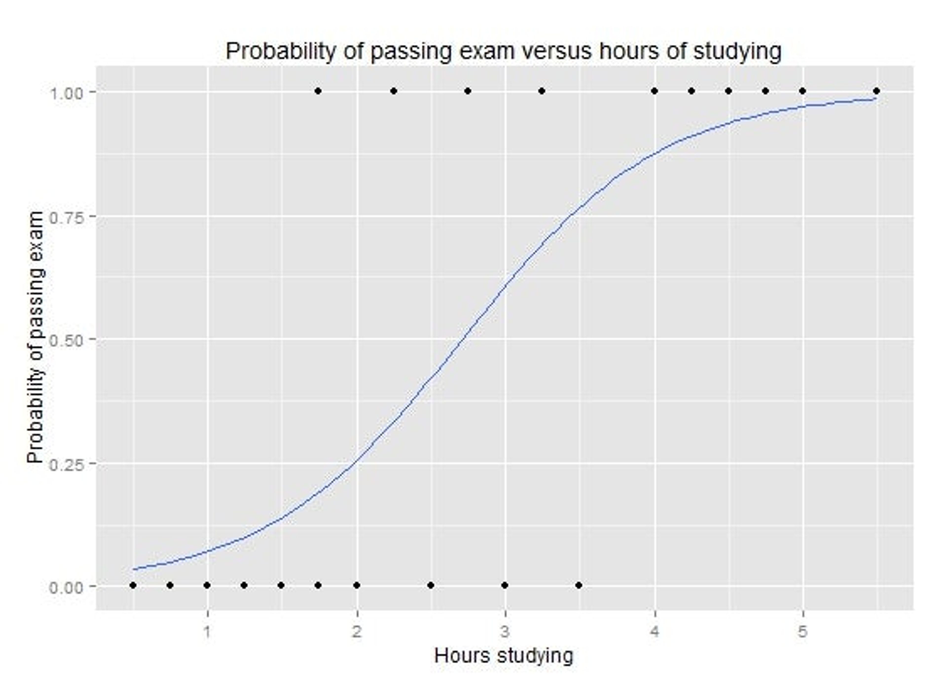
The example above, taken from the Wikipedia article on Logistic Regression, shows a plot of the probability of passing an exam relative to the hours spent studying. Logistic regression is a good technique for solving this problem because we are attempting to determine pass/fail, a binary selector. If we wanted to determine a grade or percentage on the test, simple regression would be a better technique.
To demonstrate logistic regression and how it can be used in conjunction with Redis, we will explore another classic data set, the Fisher Iris Plant Data Set.
Data Set
The Fisher Iris database consists of 150 data points labeled with one of 3 different species of Iris: Iris setosa, Iris versicolor, and Iris Virginica. Each data point consists of four attributes (features) of the plant. Using logistic regression, we can use the attributes to classify an Iris into one of the three species.
The Fisher Iris database is one of the data sets included in the Python scikit learn package. To load the data set, use the following code:
We can print out the data in a table and see that our data consists of sepal length, sepal width, petal length and petal width, all in centimeters.
Our target classification is encoded as integer values 0, 1, and 2. A 0 corresponds to Iris Setosa, a 1 corresponds to Iris Versicolor and a 2 corresponds to an Iris Virginica.

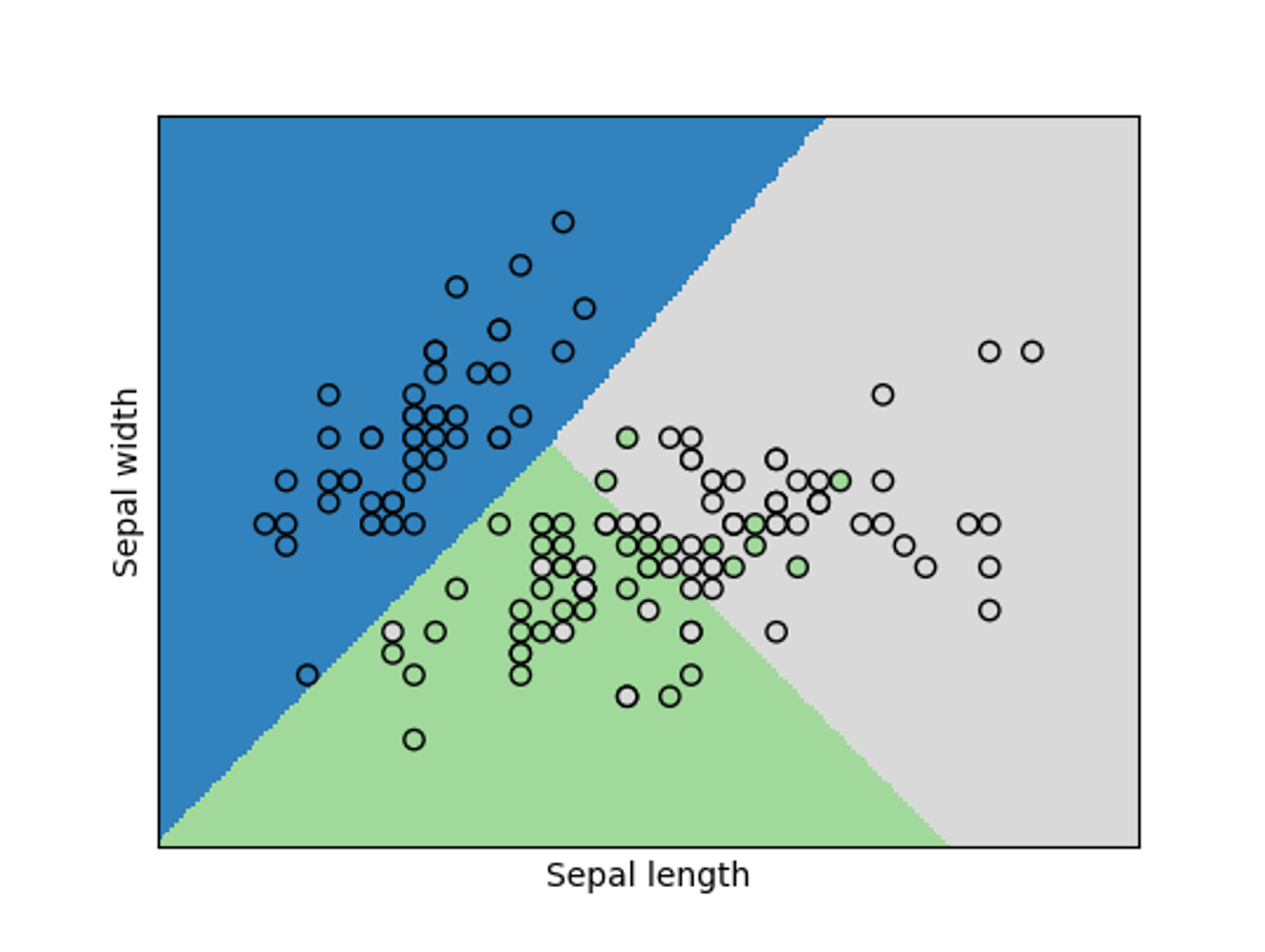
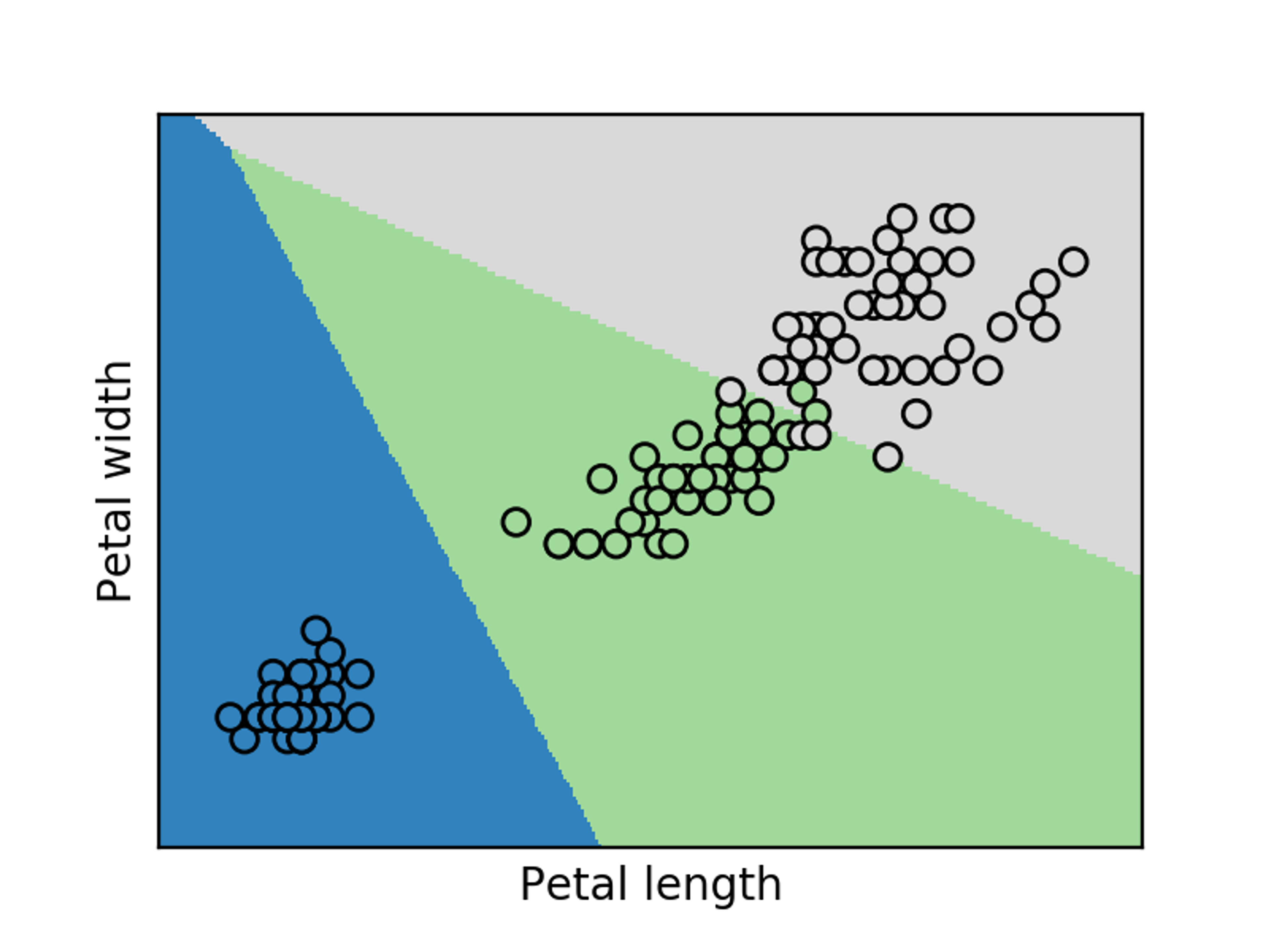
To get a better sense of the relationship between various measurements and the flower type, we generated two plots: one of sepal width versus length and another of petal width versus length. Each graph shows the classification boundaries (determined through logistic regression) of the three classes and overlays it with the points from our data set. Blue represents the area classified as Iris setosa, green represents Iris versicolor and grey represents Iris Virginica:

We can see in both plots that there are a few outliers that get misclassified, but most of our Iris types cluster together in distinct groups.
Performing a Logistic Regression
The code to perform a logistic regression in scikit is similar to the code we used previously to perform a linear regression. We first need to create our training and test sets, then we fit a logistic regression.
To split the training and test sets, we use the following code:
For this example, we split our data into blocks of 10 elements, put the first element into the test set and put the remaining 9 elements into the training set. To ensure our data contains selections from all three classes, we’ll need to use a more involved process in this example than previous examples.
Once we construct our training and test sets, fitting the logistic regression requires two lines of code:
The final line of code uses our trained logistic regression to predict the Iris types of our test set.
Redis Predictor
As with our linear regression example, we can build a logistic regression predictor using Redis.
The Redis-ML module provides ML.LOGREG.SET and ML.LOGREG.PREDICT functions to create logistic regression keys.
To add a logistic regression model to Redis, you need to use the ML.LOGREG.SET command to add the key to the database. The ML.LOGREG.SET command has the following form:
and the ML.LOGREG.PREDICT function is used to evaluate the logistic regression from the feature values and has the form:
The order of the feature values in the PREDICT command must correspond to the coefficients. The result of the PREDICT command is the probability that an observation belongs to a particular class.
To use Redis to construct a multiclass classifier, we have to emulate the One vs. Rest procedure used for multiclass classification. In the One vs. Rest procedure, multiple classifiers are created, each used to determine the probability of an observation being in a particular class. The observation is then labeled with the class it is most likely to be a member of.
For our three-class Iris problem, we will need to create three separate classifiers, each determining the probability of a data point being in that particular class. The scikit LogisticRegression object defaults to One vs. Rest (ovr in the scikit API) and fits the coefficients for three separate classifiers.
To emulate this procedure in Redis, we first create three logistic regression keys corresponding to the coefficients fit by scikit:
We emulate the One vs. Rest prediction procedure that takes place in the LogisticRegression.predict function by iterating over our three keys and then taking the class with the highest probability. The following code executes the One vs. Rest procedure over our test data and stores the resulting labels in a vector:
We compare the final classifications by printing out the three result vectors:
The output vectors show the actual Iris species (y_test) and the predictions made by scikit (y_pred) and Redis (r_pred). Each vector stores the output as an ordered sequence of labels, encoded as integers.
Redis and scikit made identical predictions, including the mislabeling of one Virginica as a Versicolor.
You may not have a need for a highly-available, real-time Iris classifier, but by leveraging this classic data set you’ve learned how to use the Redis-ML module to implement a highly available, real-time classifier for your own data.
In the next post, we’ll continue our examination of the features of the Redis-ML module by looking at the matrix operations supported by Redis-ML and how they can be used to solve ML problems. Until then, if you have any questions regarding these posts, connect with the author on twitter (@tague).
Get started with Redis today
Speak to a Redis expert and learn more about enterprise-grade Redis today.
